msepred

Predicted mean squared error for LMS adaptive filter

Syntax

[mmseemse] = msepred(lmsFilt,x,d)

[mmseemse,meanw,mse,tracek] = msepred(lmsFilt,x,d)

[mmseemse,meanw,mse,tracek] = msepred(lmsFilt,x,d,m)

Description

[mmseemse] = msepred(lmsFilt,x,d) predicts the steady-state values at convergence of the minimum mean squared error, mmse, and the excess mean squared error, emse, given the input and the desired response signal sequences in x and d and the quantities in the dsp.LMSFilter System object™, lmsFilt.

[mmseemse,meanw,mse,tracek] = msepred(lmsFilt,x,d) also computes meanw, the sequence of means of the coefficient vectors, mse, sequence of mean-squared errors, and tracek, the sequence of total coefficient error powers.

[mmseemse,meanw,mse,tracek] = msepred(lmsFilt,x,d,m) specifies an optional decimation factor for computing meanw, mse, and tracek. If m > 1, every m^th predicted value of each of these sequences is saved. If omitted, the value of m is the default, which is one.

Examples

Predict Mean Squared Error for LMS Filter

The mean squared error (MSE) measures the average of the squares of the errors between the desired signal and the primary signal input to the adaptive filter. Reducing this error converges the primary input to the desired signal. Determine the predicted value of MSE and the simulated value of MSE at each time instant using the msepred and msesim functions. Compare these MSE values with each other and with respect to the minimum MSE and steady-state MSE values. In addition, compute the sum of the squares of the coefficient errors given by the trace of the coefficient covariance matrix.

Initialization

Create a dsp.FIRFilter System object™ that represents the unknown system. Pass the signal, x, to the FIR filter. The output of the unknown system is the desired signal, d, which is the sum of the output of the unknown system (FIR filter) and an additive noise signal, n.

num = fir1(31,0.5);
fir = dsp.FIRFilter('Numerator',num);  
iir = dsp.IIRFilter('Numerator',sqrt(0.75),...
        'Denominator',[1 -0.5]);
x = iir(sign(randn(2000,25))); 
n = 0.1*randn(size(x));           
d = fir(x) + n; 

LMS Filter

Create a dsp.LMSFilter System object to create a filter that adapts to output the desired signal. Set the length of the adaptive filter to 32 taps, step size to 0.008, and the decimation factor for analysis and simulation to 5. The variable simmse represents the simulated MSE between the output of the unknown system, d, and the output of the adaptive filter. The variable mse gives the corresponding predicted value.

l = 32;
mu = 0.008;
m  = 5;

lms = dsp.LMSFilter('Length',l,'StepSize',mu);
[mmse,emse,meanW,mse,traceK] = msepred(lms,x,d,m);
[simmse,meanWsim,Wsim,traceKsim] = msesim(lms,x,d,m);

Plot the MSE Results

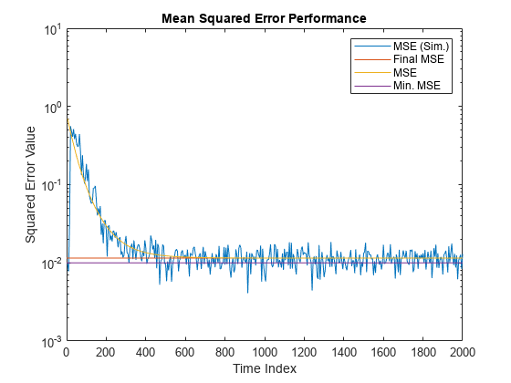
Compare the values of simulated MSE, predicted MSE, minimum MSE, and the final MSE. The final MSE value is given by the sum of minimum MSE and excess MSE.

nn = m:m:size(x,1);
semilogy(nn,simmse,[0 size(x,1)],[(emse+mmse)...
    (emse+mmse)],nn,mse,[0 size(x,1)],[mmse mmse])
title('Mean Squared Error Performance')
axis([0 size(x,1) 0.001 10])
legend('MSE (Sim.)','Final MSE','MSE','Min. MSE')
xlabel('Time Index')
ylabel('Squared Error Value')

The predicted MSE follows the same trajectory as the simulated MSE. Both these trajectories converge with the steady-state (final) MSE.

Plot the Coefficient Trajectories

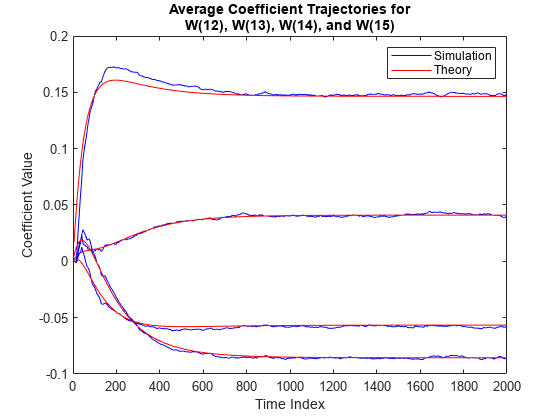
meanWsim is the mean value of the simulated coefficients given by msesim. meanW is the mean value of the predicted coefficients given by msepred.

Compare the simulated and predicted mean values of LMS filter coefficients 12,13,14, and 15.

plot(nn,meanWsim(:,12),'b',nn,meanW(:,12),'r',nn,...
meanWsim(:,13:15),'b',nn,meanW(:,13:15),'r')
PlotTitle ={'Average Coefficient Trajectories for';...
            'W(12), W(13), W(14), and W(15)'}

PlotTitle = 2×1 cell
    {'Average Coefficient Trajectories for'}
    {'W(12), W(13), W(14), and W(15)'      }

title(PlotTitle)
legend('Simulation','Theory')
xlabel('Time Index')
ylabel('Coefficient Value')

In steady state, both the trajectories converge.

Sum of Squared Coefficient Errors

Compare the sum of the squared coefficient errors given by msepred and msesim. These values are given by the trace of the coefficient covariance matrix.

semilogy(nn,traceKsim,nn,traceK,'r')
title('Sum-of-Squared Coefficient Errors')
axis([0 size(x,1) 0.0001 1])
legend('Simulation','Theory')
xlabel('Time Index')
ylabel('Squared Error Value')

Input Arguments

lmsFilt — LMS adaptive filter System object

dsp.LMSFilter

LMS adaptive filter, specified as a dsp.LMSFilter System object.

x — Input signal

scalar | column vector | matrix

Input signal, specified as a scalar, column vector, or matrix. Columns of the matrix x contain individual input signal sequences. The input, x, and the desired signal, d, must have the same size, data type, and complexity.

Data Types: single | double

d — Desired signal

scalar | column vector | matrix

Desired response signal, specified as a scalar, column vector, or matrix. Columns of the matrix d contain individual desired signal sequences. The input, x, and the desired signal, d, must have the same size, data type, and complexity.

Data Types: single | double

m — Decimation factor

1 (default) | positive scalar

Decimation factor, specified as a positive scalar. Every mth predicted value of the 3rd, 4th, and 5th predicted sequences output is saved into the corresponding output arguments, meanw, mse, and tracek. If m equals 1, every value of these sequences is saved.

m must be a factor of the input frame size.

Data Types: single | double | int8 | int16 | int32 | int64 | uint8 | uint16 | uint32 | uint64 | logical

Output Arguments

mmse — Minimum mean squared error

scalar

Minimum mean squared error (mmse), returned as a scalar. This parameter is estimated using a Wiener filter. The Wiener filter minimizes the mean squared error between the desired signal and the input signal filtered by the Wiener filter. A large value of the mean squared error indicates that the adaptive filter cannot accurately track the desired signal. The minimal value of the mean squared error ensures that the adaptive filter is optimal. The minimum mean squared error between a particular frame of the desired signal and the filtered signal is computed as the variance between the two frames of signals. The msepred function outputs the average of the mmse values for all the frames. For more details on how this parameter is calculated, see Algorithms.

Data Types: single | double

emse — Steady state excess mean squared error

scalar

Excess mean squared error, returned as a scalar. This error is the difference between the mean squared error introduced by adaptive filters and the minimum mean squared error produced by corresponding Wiener filter. For details on how this parameter is calculated, see Algorithms.

Data Types: single | double

meanw — Sequence of coefficient vector means

matrix

Sequence of coefficient vector means of the adaptive filter at each time instant, returned as a matrix. The columns of this matrix contain predictions of the mean values of the LMS adaptive filter coefficients at each time instant. If the decimation factor, m equals 1, the dimensions of meanw is M-by-N. M is the frame size (number of rows) of the input signal, x. N is the length of the FIR filter weights vector, specified by the Length property of the lmsFilt System object. If m > 1, the dimensions of meanw is M/m-by-N.

For details on how this parameter is calculated, see Algorithms.

Data Types: double

mse — Sequence of mean squared errors

column vector

Predictions of the mean squared error of the LMS adaptive filter at each time instant, returned as a column vector. If the decimation factor, m equals 1, the length of mse equals the frame size (number of rows) of the input signal, M. If m > 1, the length of mse equals M/m.

For details on how this parameter is calculated, see Algorithms.

Data Types: double

tracek — Sequence of total coefficient error powers

column vector

Predictions of the total coefficient error power of the LMS adaptive filter at each time instant, returned as a column vector. If the decimation factor, m equals 1, the length of tracek equals the frame size (number of rows) of the input signal, given by size(x,1). If m > 1, the length of tracek equals the ratio of input frame size and the decimation factor, m.

For details on how this parameter is calculated, see Algorithms.

Data Types: double

Algorithms

Minimum Mean Squared Error (mmse)

The msepred function computes the minimum mean-squared error (mmse) using the following equation:

$$mmse=\frac{{\displaystyle \sum _{i=1}^N\mathrm{var}(d_i}-W(x_i))}{N}$$

where,

• N –– Number of frames in the input signal, x.

• d_i –– ith frame (column) of the desired signal.

• x_i –– ith frame (column) of the input signal.

• W(x_i) –– Output of the Wiener filter.

• var –– Variance

Excess Mean Squared Error (emse)

The msepred function computes the steady-state excess mean squared error using the following equations:

$$\begin{array}{l}emse=K\lambda ,\\ K=\frac{B}{I(L)-A},\\ B={\mu }^2.mmse.\lambda \text{'},\\ A=I(L)-2\mu Lam+{\mu }^2(La{m}^2(kurt+2)+\lambda \lambda \text{'}).\end{array}$$

where,

• K –– Final values of transformed coefficient variances.

• λ –– Column vector containing the eigenvalues of the input autocorrelation matrix.

• λ' –– Transpose of λ.

• B –– MSE analysis driving term.

• L –– Length of the FIR adaptive filter, given by lmsFilt.Length.

• I(L) –– L-by-L identity matrix.

• A –– MSE analysis transition matrix.

• μ –– Step size given by lmsFilt.StepSize.

• Lam –– Diagonal matrix containing the eigenvalues.

• kurt –– Average kurtosis value of eigenvector-filtered signals.

Coefficient Vector Means (meanw)

The msepred function computes each element of the sequence of coefficient vector means using the following equations:

$$\begin{array}{l}meanw=meanw.T.D,\\ T=I(L)-\mu R,\\ D=\mu P.\end{array}$$

where,

• meanw –– The initial value of meanw is given by lmsFilt.InitialConditions.

• T –– Transition matrix for mean coefficient analysis.

• I(L) –– L-by-L identity matrix.

• μ –– Step size given by lmsFilt.StepSize.

• R –– Input autocorrelation matrix of size L-by-L.

• D –– Driving term for mean coefficient analysis.

• P –– Cross correlation vector of size 1-by-L.

• kurt –– Average kurtosis value of eigenvector-filtered signals.

Mean Squared Errors (mse)

The msepred function computes each element of the sequence of the mean squared errors using the following equations:

$$\begin{array}{l}mse=mmse+dk.\lambda ,\\ dk=dk\circ diagA+mse.D,\\ diagA=(1-2\mu \lambda +{\mu }^2(kurt+2){\lambda }^{\circ 2})\text{'},\\ D={\mu }^2\lambda \text{'}.\end{array}$$

where,

• mmse –– Minimum mean squared error.

• dk –– Diagonal entries of coefficient covariance matrix. The initial value of dk is given by $$dk={((meanw-Wopt)Q)}^{\circ 2}$$.

• meanw –– Coefficient vector means given by lmsFilt.InitialConditions.

• Wopt –– Optimal Wiener filter coefficients.

• Q –– L-by-L matrix whose columns are the eigenvectors of the input autocorrelation matrix, R, so that RQ = QLam. Lam is the diagonal matrix containing the corresponding eigen values.

• diagA –– Portion of MSE analysis transition matrix.

• dk◦diagA –– Hadamard or entrywise product of dk and diagA.

• λ –– Column vector containing the eigenvalues of the input autocorrelation matrix, R.

• μ –– Step size given by lmsFilt.StepSize.

• kurt –– Average kurtosis value of eigenvector filtered signals.

• λ^◦2 –– Hadamard or entrywise power of the column vector containing the eigenvalues.

• D –– Driving term for MSE analysis.

Total Coefficient Error Powers (tracek)

The msepred function computes each element of the sequence of the total coefficient error powers. These values are given by the trace of the coefficient covariance matrix. The diagonal entries of the coefficient covariance matrix are given by dk in the following equations:

$$\begin{array}{l}mse=mmse+dk.\lambda ,\\ dk=dk\circ diagA+mse.D,\\ diagA=(1-2\mu \lambda +{\mu }^2(kurt+2){\lambda }^{\circ 2})\text{'},\\ D={\mu }^2\lambda \text{'}.\end{array}$$

The trace of the coefficient covariance matrix is given by the following equation:

$$tracek=sum(dk).$$

References

[1] Hayes, M.H. Statistical Digital Signal Processing and Modeling. New York: John Wiley & Sons, 1996.

Version History

Introduced in R2012a