spaps
Smoothing spline
Syntax
Description
Note
For a simpler but less flexible method to generate smoothing splines, try the Curve Fitter app or the fit function.
sp = spaps(x,y,tol) tol of the given data points (x(j), y(:,j)), j=1:length(x). The data values y(:,j) are scalars, vectors, matrices, or even ND-arrays. Data points with the same data site are replaced by their weighted average, with its weight the sum of the corresponding weights, and the tolerance tol is reduced accordingly.
[sp, also returns the smoothed values. values] = spaps(x,y,tol) values is the same as fnval(sp,x).
Here, the distance of the function f from the given data is measured by
with the default choice for the weights w making E(f) the composite trapezoidal rule approximation to , and |z|2 denoting the sum of squares of the entries of z.
Further, smoothest means that the following roughness measure is minimized:
where Dmf denotes the mth derivative of f. The default value for m is 2, the default value for the roughness measure weight λ is the constant 1, and this makes f a cubic smoothing spline.
When tol is nonnegative, then the spline f is determined as the unique minimizer of the expression ρE(f) + F(Dmf), with the smoothing parameter ρ (optionally returned) so chosen that E(f) equals tol. Hence, when m is 2, then, after conversion to ppform, the result should be the same (up to round-off) as obtained by csaps(x,y,ρ/(ρ + 1)). Further, when tol is zero, then the “natural” or variational spline interpolant of order 2m is returned. For large enough tol, the least-squares approximation to the data by polynomials of degree <m is returned.
When tol is negative, then ρ is -tol.
The default value for the weight function λ in the roughness measure is the constant function 1. But you can choose it to be, more generally, a piecewise constant function, with breaks only at the data sites. Assuming the vector x to be strictly increasing, you specify such a piecewise constant λ by inputting tol as a vector of the same size as x. In that case, tol(i) is taken as the constant value of λ on the interval (x(i-1) .. x(i)), i=2:length(x), while tol(1) continues to be used as the specified tolerance.
[sp,values, also returns the actual value of ρ used as the third output argument.rho] = spaps(x,y,tol)
[...] = spaps(x,y,tol, lets you specify the weight vector w,m) w and/or the integer m, by supplying them as an argi. For this, w must be a nonnegative vector of the same size as x; m must be 1 (for a piecewise linear smoothing spline), or 2 (for the default cubic smoothing spline), or 3 (for a quintic smoothing spline).
If the resulting smoothing spline, sp, is to be evaluated outside its basic interval, it should be replaced by fnxtr(sp,m) to ensure that its m-th derivative is zero outside that interval.
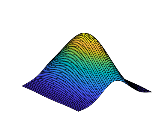
[...] = spaps({x1,...,xr},y,tol,...) returns the B-form of an r-variate tensor-product smoothing spline that is roughly within the specified tolerance to the given gridded data. For scattered data, use tpaps. Now y is expected to supply the corresponding gridded values, with size(y) equal to [length(x1),...,length(xr)] in case the function is scalar-valued, and equal to [d,length(x1),...,length(xr)] in case the function is d-valued. Further, tol must be a cell array with r entries, with tol{i} the tolerance used during the i-th step when a univariate (but vector-valued) smoothing spline in the i-th variable is being constructed. The optional input for m must be an r-vector (with entries from the set {1,2,3}), and the optional input for w must be a cell array of length r, with w{i} either empty (to indicate that the default choice is wanted) or else a positive vector of the same length as xi.
Examples
Input Arguments
Output Arguments
Algorithms
This function uses the Reinsch's approach [1] , including his way of choosing the equation for the optimal smoothing parameter in such a way that a good initial guess is available and Newton's method is guaranteed to converge and to converge fast.
References
[1] C. Reinsch. "Smoothing by spline functions." Numer. Math. 10 (1967), 177–183.
Version History
Introduced before R2006a


