bodeplot

Plot Bode frequency response with additional plot customization options

Syntax

h = bodeplot(sys)

h = bodeplot(sys1,sys2,...,sysN)

h = bodeplot(sys1,LineSpec1,...,sysN,LineSpecN)

h = bodeplot(AX,___)

h = bodeplot(___,plotoptions)

h = bodeplot(___,w)

Description

bodeplot lets you plot the Bode magnitude and phase of a dynamic system model with a broader range of plot customization options than bode. You can use bodeplot to obtain the plot handle and use it to customize the plot, such as modify the axes labels, limits and units. You can also use bodeplot to draw a Bode response plot on an existing set of axes represented by an axes handle. To customize an existing Bode plot using the plot handle:

1. Obtain the plot handle

2. Use getoptions to obtain the option set

3. Update the plot using setoptions to modify the required options

For more information, see Customizing Response Plots from the Command Line. To create Bode plots with default options or to extract the frequency response data, use bode.

h = bodeplot(sys) plots the Bode magnitude and phase of the dynamic system model sys and returns the plot handle h to the plot. You can use this handle h to customize the plot with the getoptions and setoptions commands. If sys is a multi-input, multi-output (MIMO) model, then bodeplot produces a grid of Bode plots, each plot displaying the frequency response of one I/O pair.

h = bodeplot(sys1,sys2,...,sysN) plots the frequency response of multiple dynamic systems sys1,sys2,…,sysN on the same plot. All systems must have the same number of inputs and outputs to use this syntax.

h = bodeplot(sys1,LineSpec1,...,sysN,LineSpecN) sets the line style, marker type, and color for the Bode response of each system. All systems must have the same number of inputs and outputs to use this syntax.

h = bodeplot(AX,___) plots the Bode response on the Axes or UIAxes object in the current figure with the handle AX. Use this syntax when creating apps using bodeplot in the App Designer.

h = bodeplot(___,plotoptions) plots the Bode frequency response with the options set specified in plotoptions. You can use these options to customize the Bode plot appearance using the command line. Settings you specify in plotoptions overrides the preference settings in the MATLAB^® session in which you run bodeplot. Therefore, this syntax is useful when you want to write a script to generate multiple plots that look the same regardless of the local preferences.

h = bodeplot(___,w) plots system responses for frequencies specified by the frequencies in w.

• If w is a cell array of the form {wmin,wmax}, then bodeplot plots the response at frequencies ranging between wmin and wmax.

• If w is a vector of frequencies, then bodeplot plots the response at each specified frequency.

You can use w with any of the input-argument combinations in previous syntaxes.

See logspace to generate logarithmically spaced frequency vectors.

Examples

Customize Bode Plot using Plot Handle

For this example, use the plot handle to change the frequency units to Hz and turn off the phase plot.

Generate a random state-space model with 5 states and create the Bode plot with plot handle h.

rng("default")
sys = rss(5);
h = bodeplot(sys);

Change the units to Hz and suppress the phase plot. To do so, edit properties of the plot handle, h using setoptions.

setoptions(h,'FreqUnits','Hz','PhaseVisible','off');

The Bode plot automatically updates when you call setoptions.

Alternatively, you can also use the bodeoptions command to specify the required plot options. First, create an options set based on the toolbox preferences.

p = bodeoptions('cstprefs');

Change properties of the options set by setting the frequency units to Hz and hide the phase plot.

p.FreqUnits = 'Hz';
p.PhaseVisible = 'off';
bodeplot(sys,p);

You can use the same option set to create multiple Bode plots with the same customization. Depending on your own toolbox preferences, the plot you obtain might look different from this plot. Only the properties that you set explicitly, in this example PhaseVisible and FreqUnits, override the toolbox preferences.

Custom Bode Plot Settings Independent of Preferences

For this example, create a Bode plot that uses 15-point red text for the title and sets a custom title. When you specify plot properties explicitly using bodeoptions, the specified properties override the MATLAB session preferences. Thus, the plot looks the same regardless of the preferences of the MATLAB session in which it is generated.

First, create a default options set using bodeoptions.

opts = bodeoptions;

Next, change the required properties of the options set opts. Because opt.Title is a structure, specify the properties of the plot title by specifying the fields and values of that structure.

opts.Title.FontSize = 15;
opts.Title.Color = [1 0 0];
opts.Title.String = 'System Frequency Response';
opts.FreqUnits = 'Hz';

Now, create a Bode plot using the options set opts.

bodeplot(tf(1,[1,1]),opts);

Because opts begins with a fixed set of options, the plot result is independent of the toolbox preferences of the MATLAB session.

Customized Bode Plot of Transfer Function

For this example, create a Bode plot of the following continuous-time SISO dynamic system. Then, turn the grid on, rename the plot and change the frequency scale.

$$sys(s)=\frac{s^2+0.1s+7.5}{s^4+0.12s^3+9s^2}.$$

Create the transfer function sys.

sys = tf([1 0.1 7.5],[1 0.12 9 0 0]);

Next, create the options set using bodeoptions and change the required plot properties.

plotoptions = bodeoptions;
plotoptions.Grid = 'on';
plotoptions.FreqScale = 'linear';
plotoptions.Title.String = 'Bode Plot of Transfer Function';

Now, create the Bode plot with the custom option set plotoptions.

bodeplot(sys,plotoptions)

bodeplot automatically selects the plot range based on the system dynamics.

Bode Plot with Specified Frequency Scale and Units

For this example, consider a MIMO state-space model with 3 inputs, 3 outputs and 3 states. Create a Bode plot with linear frequency scale, specify frequency units in Hz and turn the grid on.

Create the MIMO state-space model sys_mimo.

J = [8 -3 -3; -3 8 -3; -3 -3 8];
F = 0.2*eye(3);
A = -J\F;
B = inv(J);
C = eye(3);
D = 0;
sys_mimo = ss(A,B,C,D);
size(sys_mimo)

State-space model with 3 outputs, 3 inputs, and 3 states.

Create a Bode plot with plot handle h and use getoptions for a list of the options available.

h = bodeplot(sys_mimo);
p = getoptions(h)

p =

                   FreqUnits: 'rad/s'
                   FreqScale: 'log'
                    MagUnits: 'dB'
                    MagScale: 'linear'
                  MagVisible: 'on'
             MagLowerLimMode: 'auto'
                  PhaseUnits: 'deg'
                PhaseVisible: 'on'
               PhaseWrapping: 'off'
               PhaseMatching: 'off'
           PhaseMatchingFreq: 0
    ConfidenceRegionNumberSD: 1
                 MagLowerLim: 0
          PhaseMatchingValue: 0
         PhaseWrappingBranch: -180
                  IOGrouping: 'none'
                 InputLabels: [1x1 struct]
                OutputLabels: [1x1 struct]
                InputVisible: {3x1 cell}
               OutputVisible: {3x1 cell}
                       Title: [1x1 struct]
                      XLabel: [1x1 struct]
                      YLabel: [1x1 struct]
                   TickLabel: [1x1 struct]
                        Grid: 'off'
                   GridColor: [0.1500 0.1500 0.1500]
                        XLim: {3x1 cell}
                        YLim: {6x1 cell}
                    XLimMode: {3x1 cell}
                    YLimMode: {6x1 cell}

Use setoptions to update the plot with the required customization.

setoptions(h,'FreqScale','linear','FreqUnits','Hz','Grid','on');

The Bode plot automatically updates when you call setoptions. For MIMO models, bodeplot produces an array of Bode plots, each plot displaying the frequency response of one I/O pair.

Match Phase at Specified Frequency

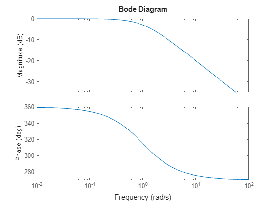
For this example, match the phase of your system response such that the phase at 1 rad/sec is 150 degrees.

First, create a Bode plot of transfer function system with plot handle h.

sys = tf(1,[1 1]); 
h = bodeplot(sys);

Use getoptions to obtain the plot properties. Change the properties PhaseMatchingFreq and PhaseMatchingValue to match a phase to a specified frequency.

p = getoptions(h); 
p.PhaseMatching = 'on'; 
p.PhaseMatchingFreq = 1; 
p.PhaseMatchingValue = 150;

Update the plot using setoptions.

setoptions(h,p);

The first bode plot has a phase of -45 degrees at a frequency of 1 rad/s. Setting the phase matching options so that at 1 rad/s the phase is near 150 degrees yields the second Bode plot. Note that, however, the phase can only be -45 + N*360, where N is an integer. So the plot is set to the nearest allowable phase, namely 315 degrees (or $$1*360-45=315^o$$).

Display Confidence Regions of Identified Models

For this example, compare the frequency responses of two identified state-space models with 2 and 6 states along with their 2 $$\sigma$$ confidence regions.

Load the identified state-space model data and estimate the two models using n4sid. Using n4sid requires a System Identification Toolbox license.

load iddata1
sys1 = n4sid(z1,2); 
sys2 = n4sid(z1,6);

Create a Bode plot of the two systems.

bodeplot(sys1,'r',sys2,'b');
legend('sys1','sys2');

From the plot, observe that both models produce about 70% fit to data. However, sys2 shows higher uncertainty in its frequency response, especially close to the Nyquist frequency. Now, use linspace to create a vector of frequencies and plot the Bode response using the frequency vector w.

w = linspace(8,10*pi,256);
h = bodeplot(sys1,sys2,w);
legend('sys1','sys2');

Use setoptions to turn on phase matching and to specify the standard deviation of the confidence region.

setoptions(h,'PhaseMatching','on','ConfidenceRegionNumberSD',2);

You can use the showconfidence command to display the confidence regions on the Bode plot.

showConfidence(h)

Frequency Response of Identified Parametric and Nonparametric Models

For this example, compare the frequency response of a parametric model, identified from input/output data, to a non-parametric model identified using the same data. Identify parametric and non-parametric models based on the data.

Load the data and create the parametric and non-parametric models using tfest and spa, respectively.

load iddata2 z2;
w = linspace(0,10*pi,128);
sys_np = spa(z2,[],w);
sys_p = tfest(z2,2);

spa and tfest require System Identification Toolbox™ software. The model sys_np is a non-parametric identified model while, sys_p is a parametric identified model.

Create an options set to turn phase matching and the grid on. Then, create a Bode plot that includes both systems using this options set.

plotoptions = bodeoptions;  
plotoptions.PhaseMatching = 'on';
plotoptions.Grid = 'on';
bodeplot(sys_p,sys_np,w,plotoptions);
legend('Parametric Model','Non-Parametric model');

Input Arguments

sys — Dynamic system

dynamic system model | model array

Dynamic system, specified as a SISO or MIMO dynamic system model or array of dynamic system models. Dynamic systems that you can use include:

• Continuous-time or discrete-time numeric LTI models, such as tf, zpk, or ss models.

• Sparse state-space models, such as sparss or mechss models. Frequency grid w must be specified for sparse models.

• Generalized or uncertain LTI models such as genss or uss (Robust Control Toolbox) models. (Using uncertain models requires Robust Control Toolbox™ software.)

  • For tunable control design blocks, the function evaluates the model at its current value to plot the frequency response data.

  • For uncertain control design blocks, the function plots the nominal value and random samples of the model.

• Frequency-response data models such as frd models. For such models, the function plots the response at frequencies defined in the model.

• Identified LTI models, such as idtf (System Identification Toolbox), idss (System Identification Toolbox), or idproc (System Identification Toolbox) models. For such models, the function can also plot confidence intervals and return standard deviations of the frequency response. See Bode Plot of Identified Model. (Using identified models requires System Identification Toolbox™ software.)

If sys is an array of models, the function plots the frequency responses of all models in the array on the same axes.

LineSpec — Line style, marker, and color

character vector | string

Line style, marker, and color, specified as a character vector or string containing symbols. The symbols can appear in any order. You do not need to specify all three characteristics (line style, marker, and color). For example, if you omit the line style and specify the marker, then the plot shows only the marker and no line.

Example: '--or' is a red dashed line with circle markers

Line Style	Description
-	Solid line
--	Dashed line
:	Dotted line
-.	Dash-dot line

Marker	Description
'o'	Circle
'+'	Plus sign
'*'	Asterisk
'.'	Point
'x'	Cross
'_'	Horizontal line
'|'	Vertical line
's'	Square
'd'	Diamond
'^'	Upward-pointing triangle
'v'	Downward-pointing triangle
'>'	Right-pointing triangle
'<'	Left-pointing triangle
'p'	Pentagram
'h'	Hexagram

Color	Description
y	yellow
m	magenta
c	cyan
r	red
g	green
b	blue
w	white
k	black

AX — Target axes

Axes object | UIAxes object

Target axes, specified as an Axes or UIAxes object. If you do not specify the axes and if the current axes are Cartesian axes, then bodeplot plots on the current axes. Use AX to plot into specific axes when creating apps in the App Designer.

plotoptions — Bode plot options set

BodePlotOptions object

Bode plot options set, specified as a BodePlotOptions object. You can use this option set to customize the Bode plot appearance. Use bodeoptions to create the option set. Settings you specify in plotoptions overrides the preference settings in the MATLAB session in which you run bodeplot. Therefore, plotoptions is useful when you want to write a script to generate multiple plots that look the same regardless of the local preferences.

For the list of available options, see bodeoptions.

w — Frequencies

{wmin,wmax} | vector

Frequencies at which to compute and plot frequency response, specified as the cell array {wmin,wmax} or as a vector of frequency values.

• If w is a cell array of the form {wmin,wmax}, then the function computes the response at frequencies ranging between wmin and wmax.

• If w is a vector of frequencies, then the function computes the response at each specified frequency. For example, use logspace to generate a row vector with logarithmically spaced frequency values.

Specify frequencies in units of rad/TimeUnit, where TimeUnit is the TimeUnit property of the model.

Output Arguments

h — Plot handle

handle object

Plot handle, returned as a handle object. Use the handle h to get and set the properties of the Bode plot using getoptions and setoptions. For the list of available options, see the Properties and Values Reference section in Customizing Response Plots from the Command Line.

Version History

Introduced before R2006a