showConfidence
Display confidence regions on response plots for identified models
Description
showConfidence( displays the
confidence region on the response plot for an identified model using a default standard
deviation of plotHandle)1.
showConfidence(
displays the confidence region for plotHandle,stdDev)sd standard deviations.
Examples
Show the confidence bounds on the bode plot of an identified ARX model.
Obtain identified model and plot its bode response.
load iddata1 z1
sys = arx(z1, [2 2 1]);
h = bodeplot(sys);
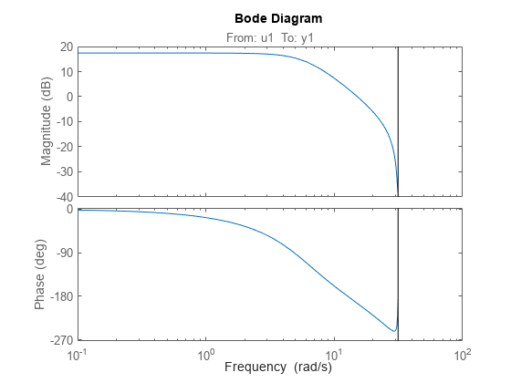
z1 is an iddata object that contains time domain system response data. sys is an idpoly model containing the identified polynomial model. h is the plot handle for the bode response plot of sys.
Show the confidence bounds for sys.
showConfidence(h);
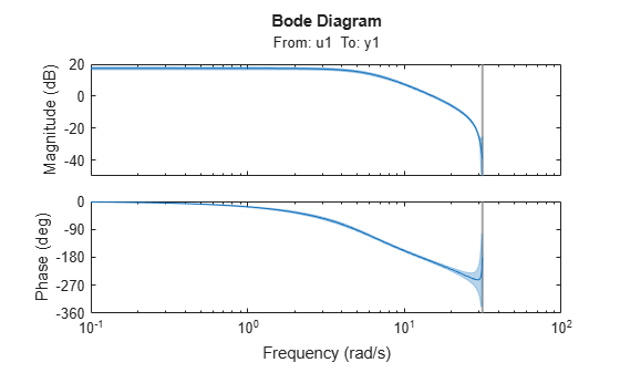
This plot depicts the confidence region for 1 standard deviation.
Show the confidence bounds on the bode plot of an identified ARX model.
Obtain identified model and plot its bode response.
load iddata1 z1
sys = arx(z1, [2 2 1]);
bp = bodeplot(sys);

z1 is an iddata object that contains time domain system response data. sys is an idpoly model containing the identified polynomial model. bp is the chart object for the bode response plot of sys.
Show the confidence bounds for sys using 2 standard deviations.
sd = 2;
showConfidence(bp,sd);
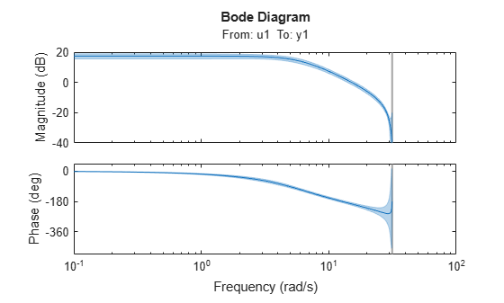
sd specifies the number of standard deviations for the confidence region displayed on the plot.
Input Arguments
Alternatives
You can interactively enable the confidence region display on a response plot. Right-click the response plot, and select Characteristics > Confidence Region.
Version History
Introduced in R2012a
See Also
bodeplot | stepplot | impulseplot | nyquistplot | iopzplot