Sinks

In Communications Toolbox™, you can assess system performance by using scopes to analyze signals. For other ways to measure system performance, see Measure Modulation Accuracy and Bit Error Rate Analysis Techniques.

The scopes enable you to plot eye diagrams or constellation diagrams and view the trajectory of a signal.

Plots	Features
Eye diagram of a signal	`eyediagram` function Eye Diagram block
Constellation diagram and trajectory of a signal	`scatterplot` function `comm.ConstellationDiagram` System object™ Constellation Diagram block

Other useful scopes for analysis of communications signals include the spectrum analyzer (spectrumAnalyzer object and Spectrum Analyzer block) and the Signal Analyzer app.

Eye Diagrams

An eye diagram is a simple and convenient tool for studying the effects of intersymbol interference, timing, noise, and other channel impairments in digital transmission. An eye diagram plots the received signal against time on a fixed-interval axis. At the end of the fixed interval, it wraps around to the beginning of the time axis. As a result, the diagram consists of many overlapping curves. One way to use an eye diagram is to look for the place where the eye is most widely opened, and use that point as the decision point when demapping a demodulated signal to recover a digital message.

For examples, see View Sinusoid in Simulink and View Modulated Signal in Simulink.

Scatter Plots and Constellation Diagrams

A scatter plot, also known as a constellation diagram, of a discrete-time signal plots the value of the signal at its decision points. In the best case, the decision points should coincide with times when the eye of the signal's eye diagram is the most widely open. The constellation diagram plots the complex-valued symbols transmitted in a digitally modulated signal, and provides a visual indication of signal to noise ratio and RF impairments.

For an example, see Visualize RF Impairments.

Signal Trajectories

A signal trajectory plots the continuous path of a discrete-time signal over time. A signal trajectory traces the path to show the sequential order of received symbols.

The constellation scope (comm.ConstellationDiagram System object or Constellation Diagram block) draws signal trajectories when you select Trajectory in Configuration on the Scope tab. A signal trajectory connects all points of the input signal, irrespective of the specified decimation factor (Samples per symbol). For an example, see View Modulated Signal in Simulink.

Scope Usage Examples

These examples demonstrate ways to use scopes for viewing eye diagrams, constellation diagrams, and signal trajectories in MATLAB^® and Simulink^®.

View Sinusoid in Simulink

This example uses:

Open Model

This example creates and displays constellation diagram and eye diagram plots of a complex sinusoidal signal in Simulink®.

The doc_eyediagram model generates a complex sinusoid with a Sine Wave block and passes it to Constellation Diagram and Eye Diagram blocks to be plotted.

model = 'doc_eyediagram';
open_system(model)

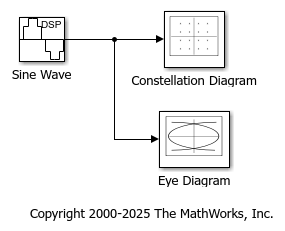
The block masks indicate the simulation configuration. To see the configuration of the Constellation Diagram or Eye Diagram block, double-click the block to open the diagram window.

The Sine Wave block sets Frequency to .502 Hz, Output complexity to Complex, Sample time to 1/16, and Samples per frame to 1024.
The Constellation Diagram block sets Samples per symbol to 16 to match the sampling time of the sine wave block, Symbols to display to 64, Color fading to selected, and Show reference constellations not selected. The Eye Diagram block sets *Samples per symbol to 16 to match the sampling time of the sine wave block, and Color fading to selected.

The eye diagram has only a Scope tab. The constellation diagram has a Scope and Measurements tab. Explore them to see the parameters available.

sim(model,'StopTime','5');

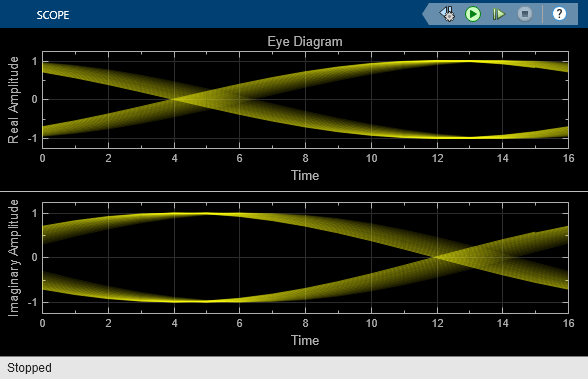
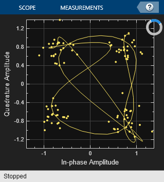
In the scatter plot, the points lie on a circle of radius 1. In the eye diagram, the upper set of traces show the real part of the signal and the lower set of traces show the imaginary part of the signal. Successive points in the scatter diagram are near each other but do not overlap. Since the color fading options is selected, the points fade as time passes. Because the decision time interval is almost, but not exactly, an integer multiple of the period of the sinusoid, the plots exhibit drift over time.

View Modulated Signal in Simulink

This example uses:

Open Model

This example creates and displays eye diagram, constellation diagram, and signal trajectory plots for a QPSK-modulated signal in Simulink®.

The doc_signaldisplays model generates a QPSK-modulated signal by using a Random Integer Generator block as the input to a QPSK Modulator Baseband block. An AWGN Channel block adds noise to the modulated signal, and a Raised Cosine Transmit Filter block filters the noisy signal. The Eye Diagram and Constellation Diagram blocks plot the filtered signal.

Block masks indicate the simulation configuration. The blocks have these parameters adjusted from the default settings.

The Random Integer Generator block adjusts Set size to 4 and Sample time to 0.01.
The QPSK Modulator Baseband block uses the default parameter settings.
The AWGN Channel block adjusts Mode to Signal-to-noise ratio (SNR) and SNR (dB) to 15.
The Raised Cosine Transmit Filter block adjusts Filter shape to Normal, Rolloff factor to 0.5, Filter span in symbols to 6, Output samples per symbol to 8, and Input processing to Elements as channels (sample based).

To plot on-time symbols, set both the Eye Diagram and Constellation diagrams to the same number as samples per symbol as output by the filter block.

Eye Diagram

The eye diagram provides a visual indication of timing, noise, and intersymbol interference. To see the configuration of the Eye Diagram block, double-click the block to open the diagram window. Under Configuration on the Scope tab, open Settings. The example sets:

Samples per symbol to 8 to match the filter block.
Symbols per trace to 3. This parameter specifies the number of symbols that are displayed in each trace of the eye diagram. A trace is any one of the individual lines in the eye diagram.
Traces to display to 3.
Color fading to selected.
Plot imaginary axis to not selected.

Simulate the model with a stop time of 90 ms. The eye diagram displays traces that vary depending on when you start the simulation. The three traces displayed vary in weight because color fading is selected. The most recent trace is the most opaque. The oldest trace is the most faded. The most recent trace contains 24 points because it plots three symbols and each symbol contains eight samples. Earlier traces have one more point because each earlier trace ends with the last point of the trace plotted after it. These duplicate points indicate where the traces would meet if they were displayed side by side.

To view a more realistic eye diagram, increase the value of Traces to display to 40. Run the simulation for 1.2 s.

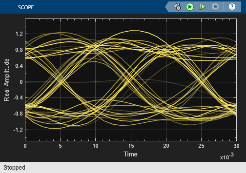
Setting the Offset parameter to 0 starts the plot at the center of the first symbol, which locates the open part of the eye diagram in the middle of the plot for most points.

Constellation Diagram

To configure the Constellation Diagram block, double-click the block to open the diagram window. Under Configuration on the Scope tab, open Settings. The example sets:

Samples per symbol to 8 to match the filter block.
Offset to 0. This parameter specifies the number of samples to skip before plotting the first point.
Symbols to display to 40.
Color fading to selected.

Simulate the model with a stop time of 1.6 s.

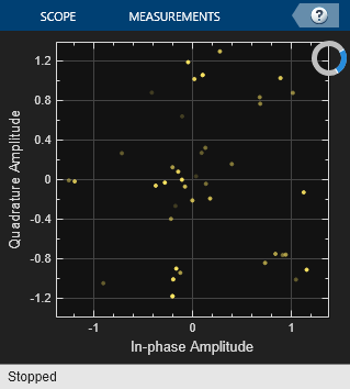
Signal Trajectory

The constellation diagram signal trajectory shows the path a modulated signal takes from symbol to symbol in the complex plane. To display the reference constellation and signal trajectory, go to Configuration in the Scopes tab of the constellation diagram window, and select Reference Constellation and Trajectory. Also, deselect color fading.

Run the simulation with a stop time of 3.2 s.

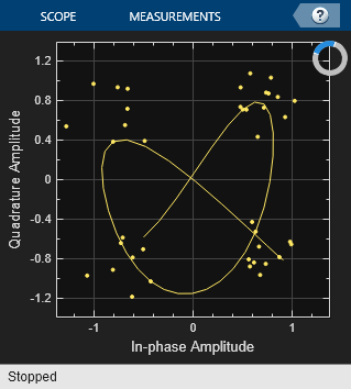
Increase the value of Symbols to display to 100. This value produces a signal trajectory with 800 points, which is the product of the Samples per symbol and Samples to display properties.

Run the simulation for 8 s.