Digital Baseband Modulation
In most media for communication, only a fixed range of frequencies is available for transmitting messages. One way to communicate a message whose frequency spectrum does not fall within that fixed frequency range, or one that is otherwise unsuitable for the channel, is to alter a carrier signal according to the information in your message signal. This alteration is called modulation. The transmitter sends the modulated symbols. The receiver then recovers the original message symbols through a process called demodulation.
Modulation Methods
Digital baseband modulation modulates digital transmission symbols into sinusoidal waveforms. Communications Toolbox™ software provides features to apply a variety of digital baseband modulation methods. The process by which a carrier signal is altered according to information in a message signal depends on the modulation method applied. The general form of the carrier signal, s(t) is
s(t) = A(t)cos[2πf0t+ϕ(t)]
The information-carrying component is the amplitude (A), frequency (f0), or phase (ϕ) individually, or in combination.
| Digital Modulation Type | Modulation Methods |
|---|---|
Pulse amplitude modulation (PAM) Quadrature amplitude modulation (QAM) | |
Amplitude and pulse shift keying (APSK) MIL-188-QAM | |
Continuous-phase frequency shift keying (CPFSK) Continuous-phase modulation (CPM) Gaussian minimum shift keying (GMSK) Minimum shift keying (MSK) | |
Frequency shift keying (FSK) | |
Orthogonal frequency division multiplexing (OFDM) | |
Phase shift keying (PSK) Differential phase shift keying (DPSK) Offset quadrature phase shift keying (OQPSK) | |
Trellis-coded modulation (TCM) Phase shift keying — TCM (PSK-TCM) Quadrature amplitude modulation — TCM (QAM-TCM) |
Note
Modulation is often followed by pulse shaping, and demodulation is often preceded by a filtering or an integrate-and-dump operation. Unless otherwise indicated, these modulation techniques do not perform pulse shaping or filtering. For examples, see Modulation with Pulse Shaping and Filtering Examples.
Modeling Concepts
Digital and analog modulation alter a transmittable signal according to the information in message symbols. Digital modulation restricts the message signal to a finite set of symbols and outputs the complex envelope of the modulated signal.
Baseband vs. Passband Simulation
Modulation is a process by which a carrier signal is altered according to information in a message signal. To recover the message through a demodulator correctly, the Nyquist sampling theorem requires fs > 2(fc + f), where fs represents the simulation sampling rate, fc represents the carrier frequency, and f represents the highest frequency of the message signal. Typically, fc >> f.
Modulation can be modeled in baseband or passband simulations. Baseband simulation, also known as the lowpass equivalent method, requires less computation.
Note
While Communications Toolbox software supports baseband simulation for digital as well as analog modulation, it supports passband simulation only for analog modulation.
When simulating baseband modulation to produce the complex envelope of the
modulated message signal, the output signal y is a
complex-valued signal related to the output of an
analog passband modulator. If the modulated passband signal has the
waveform
where fc is the carrier frequency and ϕ is the initial phase of the carrier signal, then a baseband simulation recognizes that this equals the real part of
The baseband simulation models only the part inside the square brackets. Here,
j is the square root of –1. The baseband modulated signal
vector y is a sampling of the complex signal
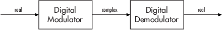
As this figure shows,
Digital modulators accept real-valued input bit vectors (or symbols) and return complex-valued output signals (or samples).
Digital demodulators accept complex-valued input signals (or samples) and return real-valued output bit vectors (or symbols).
If you want to separate the in-phase and quadrature components of the
complex modulated signal, you can use the Complex to Real-Imag (Simulink) block,
or the real and imag
MATLAB® functions.
As appropriate for a given modulation method, you can visualize the complex modulated signal by viewing the:
Modulated samples in a constellation plot
Phase tree in an eye diagram
Frequency response in a spectrum analyzer
Note
If you prefer to work with analog passband signals instead of baseband signals, then you can build functions that convert between the two. Be aware that analog passband modulation tends to be more computationally intensive than baseband modulation because the carrier signal typically needs to be sampled at a high rate.
Representing Digital Signals
To modulate a single-channel message using digital modulation, begin with a real message whose values are integers in the range [0, (M–1)], where M represents the modulation order for an M-symbol alphabet. Represent a single-channel message in a column vector or as a multichannel message in a matrix, where each column of the matrix represents one channel. For example, to modulate using an eight symbol alphabet:
The column vector
[2 3 7 1 0 5 5 2 6]'is a valid single-channel input to the modulator.The two-column matrix
[2 3; 3 3; 7 3; 0
                                        3;]
is a valid multichannel input to the modulator. The matrix for this multichannel input message specifies a second channel that has a constant value of3.
For more information, see Signal Terminology.
Integer-Valued and Binary-Valued Symbols
Most digital modulation functions, System objects, and blocks can accept either integer-valued or binary-valued symbols. For modulators, you specify the input type as integer or binary. For demodulators, you specify the output type as integer or binary.
When you configure the modulator for integer-valued input symbols, the modulator accepts integer values in the range [
0, (M–1)]. M represents the modulation order.When you configure the modulator for bit-valued input symbols, the modulator accepts binary-valued inputs that represent integers. The modulator collects binary-valued symbols into groups of b = log2(M) bits, where b represents the number of bits per symbol. The input vector length must be an integer multiple of b. In this configuration, the modulator maps groups of b bits onto symbols at the modulator output. The modulator outputs one modulated symbol for each group of b bits.
Symbol Mapping
Symbol mapping specifies the order used by the modulator to map a group of b input bits to a corresponding phasor symbol of the constellation diagram. To achieve the lower bound limit for the bit error rate, multilevel modulation schemes typically utilize the Gray coding technique. Gray-coding orders modulation symbols so that the binary representations of adjacent symbols differ by only one bit. Combining Gray-coded ordering in communications systems with forward error correction techniques capable of correcting single-bit errors helps to minimize the bit error rate in multilevel modulation schemes. For examples that demonstrate the symbol mapping and error rate performance of Gray-coding and binary-coding, see Symbol Mapping Examples.
Most of the Communications Toolbox software modulation features use Gray-coded symbol mapping as the default setting. The other symbol mapping options are binary-coded and custom-coded. The property or parameter name used for the symbol mapping input control differs as appropriate for the specific modulation method being used.
To illustrate the ordering, this table shows the relationship between 8-PSK modulated phasors output versus the corresponding modulator integer or binary symbol input values when symbol mapping uses Gray-encoding and binary-encoding.
| 8-PSK Modulator Output | Gray-Encoding | Binary-Encoding | ||
|---|---|---|---|---|
| Modulator Integer Input | Modulator Binary Input | Modulator Integer Input | Modulator Binary Input | |
exp(0) | 0 | 000 | 0 | 000 |
exp(jπ/4) | 1 | 001 | 1 | 001 |
exp(jπ/2) =
exp(j2π/4) | 3 | 011 | 2 | 010 |
exp(j3π/4) | 2 | 010 | 3 | 011 |
exp(jπ) =
exp(j4π/4) | 6 | 110 | 4 | 100 |
exp(j5π/4) | 7 | 111 | 5 | 101 |
exp(j3π/2) =
exp(j6π/4) | 5 | 101 | 6 | 110 |
exp(j7π/4) | 4 | 100 | 7 | 111 |
This constellation diagram plots the output phasors labeled with the Gray-coded values for the 8-PSK modulated symbols. Comparing to the table, you can see the row entries for Gray-encoding appear in counterclockwise order in the constellation diagram and show that there is only a 1 bit difference between neighboring samples.
Error Rate Performance of Gray-Coded M-PSK Modulation. You can analyze the data to compare theoretical performance with simulation performance. The theoretical symbol error probability of M-PSK modulation is
where erfc is the complementary error function,
Es/N0
is the ratio of energy in a symbol to noise power spectral density, and
M is the modulation order.
To determine the bit error probability, the symbol error probability, PE, needs to be converted to its bit error equivalent. There is no general formula for the symbol to bit error conversion. Upper and lower limits are nevertheless easy to establish. The actual bit error probability, Pb, can be shown to be bounded by
The lower limit corresponds to the case where the symbols have undergone Gray coding. The upper limit corresponds to the case of binary coding. Similar error rate performance improvements with Gray-coded symbol mapping applies for other modulation methods. For more information on symbol error rate (SER) and bit error rate (BER) analytical expressions, see Analytical Expressions Used in BER Analysis.
Signal Upsampling and Rate Changes
Some digital modulation methods can output an upsampled version of the modulated symbols. The corresponding digital demodulation method can accept an upsampled version of the modulated symbols as input. The samples per symbol control represents the upsampling factor and must be a positive integer. This table lists the modulation methods that offer upsampling support.
| Digital Modulation Type | Modulation Methods |
|---|---|
| Continuous-Phase Modulation | Continuous-phase frequency shift keying (CPFSK) Continuous-phase modulation (CPM) Gaussian minimum shift keying (GMSK) Minimum shift keying (MSK) |
| Frequency Modulation | Frequency shift keying (FSK) |
| Phase Modulation | Offset quadrature phase shift keying (OQPSK) |
Upsampling results in an input-to-output :
Size change for single-rate processing.
Rate change for multirate processing in Simulink®. Multirate processing is not a consideration for MATLAB.
In Simulink, your simulation can run with the rate option set for single-rate processing or multirate processing.
For more information about rate changes, see Sample- and Frame-Based Concepts.
This table summarizes the resulting upsampled output based on the processing rate option and the number of samples per symbol (NSPS) for modulation and demodulation in your simulation.
| Computation Type | Rate Option | Upsampled Output |
|---|---|---|
| Modulation | Single-rate processing | For CPM and FM — Output vector length is NSPS times the number of integers or binary words in the input vector. Output sample time equals the input sample time. For OQPSK — Output vector length is 2NSPS times the number of integers or binary words in the input vector. |
| Multirate processing | For CPM and FM — Output vector is same size as input vector. Output sample time is 1/NSPS times the input sample time. For OQPSK — Output vector is a scalar. Output sample time is 1/2NSPS times the input sample time. | |
| Demodulation | Single-rate processing | For CPM and FM — Number of integers or binary words in the output vector is 1/NSPS times the number of samples in the input vector. Output sample time equals the input sample time. For OQPSK — Output vector is 1/2NSPS times the number of samples in the input vector. |
| Multirate processing | For CPM and FM — Output vector is same size as input vector. Output sample time is NSPS times the input sample time.
For OQPSK — Output signal contains one integer or one binary word. Output sample time is 2NSPS times the input sample time. The demodulated signal is delayed by one output symbol period if NSPS > 1. |
Delays in Digital Demodulation
Some digital demodulation techniques incur delays between their inputs and outputs. These delays depend on the configuration of the demodulation techniques, and the characteristics of the modulated signals. As a result of delays, data that enters a modulation or demodulation feature at time T appears in the output at time T + delay. In particular, if your simulation computes error statistics or compares transmitted data with received data, the simulation must account for the delay when performing such computations or comparisons. For examples, see Demodulation Delay Examples.
| Demodulation Type | Situation in Which Delay Occurs | Amount of Delay |
|---|---|---|
| FM demodulator listed in Frequency Modulation | Sample-based processing | delay = One output period |
| All demodulator objects and blocks listed in Continuous-Phase Modulation | Single-rate processing, D = traceback depth value | delay = D output periods |
Blocks configured for multirate processing and if the
model uses a variable-step solver or a fixed-step solver
with the Tasking Mode parameter set to
D = Traceback length value | delay = D+1 output periods | |
| OQPSK demodulator listed in Phase Modulation | Single-rate processing | OQPSK demodulation delay varies depending
on the pulse shaping filter and the input/output settings.
For more information, see |
Blocks configured for multirate processing, and the model
uses a fixed-step solver with Tasking Mode
parameter set to Auto or
MultiTasking | ||
Blocks configured for multirate processing, and the model
uses a variable-step solver or the Tasking
Mode parameter is set to Single
Tasking | ||
| All demodulator objects and blocks listed in Trellis-Coded Modulation | Configured for continuous operation with Tr equal to the traceback depth value, and code rate k/n | delay = Tr × k output bits |
Note
Other sources of delays come from the M-DPSK, DQPSK, and DBPSK demodulators.
These demodulators produce output whose first sample is unrelated to the input.
This delay is related to the differential modulation technique, not the
particular implementation of it. To account for the delay, specify a one sample
computation delay in the error rate calculation. For an example, see comm.DQPSKDemodulator.
Hard- vs. Soft-Decision Demodulation
All Communications Toolbox demodulator functions, System objects, and blocks can demodulate binary data using hard-decisions. Some of the demodulator functions, System objects, and blocks can also demodulate binary data using soft-decisions.
The hard-decision demodulation computes the minimum Hamming distance for each received sample and selects the symbol with minimum distance. When the hard decision output for a symbol has an equal Hamming distance for multiple codewords, one of those codewords is randomly selected. Using soft-decision demodulation can reduce the probability of decision error, but it is more computationally intensive.
Two soft-decision algorithms are available: exact log-likelihood ratio (LLR) and approximate LLR. Exact LLR provides the greatest accuracy but is slower, while approximate LLR is less accurate but more efficient. For examples, see Hard- vs. Soft-Decision Demodulation Examples.
The exact LLR algorithm computes exponentials using finite precision arithmetic. For computations involving very large positive or negative magnitudes, the exact LLR algorithm yields:
Infor-Infif the noise variance is a very large valueNaNif the noise variance and signal power are both very small values
The approximate LLR algorithm does not compute exponentials. You can avoid
Inf, -Inf, and NaN results by using
the approximate LLR algorithm.
Exact LLR Algorithm
The log-likelihood ratio (LLR) is the logarithm of the ratio of probabilities of a 0 bit being transmitted versus a 1 bit being transmitted for a received signal. The LLR for a bit, b, is defined as:
Assuming equal probability for all symbols, the LLR for an AWGN channel can be expressed as:
Noise components along the in-phase and quadrature axes are assumed to be independent and of equal power, that is, .
Variables represent the values described in this table.
| Variable | Description |
|---|---|
| Received signal with coordinates (x, y) |
| Transmitted bit (one of the K bits in an M-ary symbol, assuming all M symbols are equally probable) |
| Ideal symbols or constellation points with bit 0, at the given bit position |
| Ideal symbols or constellation points with bit 1, at the given bit position |
| In-phase coordinate of ideal symbol or constellation point |
| Quadrature coordinate of ideal symbol or constellation point |
| Noise variance of baseband signal |
| Noise variance along in-phase axis |
| Noise variance along quadrature axis |
Approximate LLR Algorithm
Approximate LLR is computed by using only the nearest constellation point to the received sample with a 0 (or 1) at that bit position, rather than all the constellation points as done in exact LLR. It is defined in [8] as:
Accessing Digital Modulation Blocks
Open the Digital Baseband Modulation sublibrary by double-clicking its icon in the Modulation library.
This table lists the sublibraries in the Digital Baseband Modulation sublibrary. Double-click the icons in the Digital Baseband Modulation sublibrary to view the blocks in each individual sublibrary.
| Icon in Digital Baseband Library | Kind of Modulation |
|---|---|
| APSK | Amplitude and phase modulation |
| CPM (MSK, GMSK) | Continuous phase modulation |
| FSK | Frequency-shift keying modulation |
| OFDM | Orthogonal frequency division modulation |
| PAM/QAM | Phase amplitude and quadrature amplitude modulations |
| PSK | Phase-shift keying modulation |
| Standard-Compliant (MIL188) | MIL-STD-188 Standard-compliant modulation |
| TCM | Trellis-coded modulation |
This table lists general modulator blocks along with the conditions under which is general modulator is equivalent to a specific-case modulator block. The situation is analogous for demodulators. The specific-case modulation blocks use the same computational code that their general counterparts use, but provide an interface that is either simpler or more suitable for the specific case.
| General Modulator | General Modulator Conditions | Specific-case Modulator |
|---|---|---|
| General QAM Modulator Baseband | Predefined constellation containing M = 2b points on a rectangular lattice. M is the modulation order and b is the number of bits per symbol represented by each constellation point. | Rectangular QAM Modulator Baseband |
| M-PSK Modulator Baseband | M-ary number parameter set to
2. | BPSK Modulator Baseband |
M-ary number parameter set to
4. | QPSK Modulator Baseband | |
| M-DPSK Modulator Baseband | M-ary number parameter set to
2. | DBPSK Modulator Baseband |
M-ary number parameter set to
4. | DQPSK Modulator Baseband | |
| CPM Modulator Baseband | M-ary number parameter set to
2 and Frequency pulse
shape parameter set to
Gaussian. | GMSK Modulator Baseband |
M-ary number parameter set to 2,
Frequency pulse shape parameter set to
Rectangular, and Pulse
length parameter set to
1. | MSK Modulator Baseband | |
Frequency pulse shape parameter set to
Rectangular and Pulse
length parameter set to
1. | CPFSK Modulator Baseband | |
| General TCM Encoder | Predefined signal constellation containing M = 2b points on a rectangular lattice. | Rectangular QAM TCM Encoder |
| Predefined signal constellation containing M = 2b points on a circle. | M-PSK TCM Encoder |
The CPFSK Modulator Baseband block is similar to the M-FSK Modulator Baseband block, when the M-FSK block uses continuous phase transitions. However, the M-FSK features differ from the CPFSK features in their mask interfaces and in the demodulator implementations.
References
[1] Jeruchim, Michel C., Philip Balaban, and K. Sam Shanmugan. Simulation of Communication Systems. Second edition. Boston, MA: Springer US, 2000.
[2] Proakis, John G. Digital Communications. 5th ed. New York: McGraw Hill, 2007.
[3] Sklar, Bernard. Digital Communications: Fundamentals and Applications. Englewood Cliffs, NJ: Prentice-Hall, 1988.
[4] Anderson, John B., Tor Aulin, and Carl-Erik Sundberg. Digital Phase Modulation. New York: Plenum Press, 1986.
[5] Biglieri, E., D. Divsalar, P.J. McLane, and M.K. Simon. Introduction to Trellis-Coded Modulation with Applications. New York: Macmillan, 1991.
[6] Pawula, R.F. "On M-ary DPSK Transmission Over Terrestrial and Satellite Channels." IEEE® Transactions on Communications 32 (July 1984): 752–61.
[7] Smith, J. G. "Odd-Bit Quadrature Amplitude-Shift Keying." IEEE Transactions on Communications 23, no. 3 (March 1975): 385–89.
[8] Viterbi, A.J. “An Intuitive Justification and a Simplified Implementation of the MAP Decoder for Convolutional Codes.” IEEE Journal on Selected Areas in Communications 16, no. 2 (February 1998): 260–64. https://doi.org/10.1109/49.661114.
See Also
Topics
- Symbol Mapping Examples
- Demodulation Delay Examples
- Modulation with Pulse Shaping and Filtering Examples
- Hard- vs. Soft-Decision Demodulation Examples
- What Is Modulation?
- Amplitude Modulation
- Amplitude and Phase Modulation
- Continuous-Phase Modulation
- Frequency Modulation
- Orthogonal Frequency Division Multiplexing Modulation
- Phase Modulation
- Trellis-Coded Modulation
- Analog Passband Modulation
- Analog Baseband Modulation