Amplitude and Phase Modulation Examples
These examples demonstrate amplitude and phase modulation techniques.
Apply APSK Modulation Modifying Symbol Ordering
Plot APSK constellations for Gray-coded and custom-coded symbol mappings.
Define vectors for modulation order and PSK ring radii. Generate bit data for constellation points.
M = [8 8];
modOrder = sum(M);
radii = [0.5 1.5];
x = 0:modOrder-1;
The apskmod function assumes the single channel binary input is left-MSB aligned and specified column-wise. Use the int2bit function to express the integer input symbols as a single column binary vector.
xBit = int2bit(x,log2(modOrder));
Apply APSK modulation to the data using the default phase offset. Since element values for M are equal and element values for phase offset are equal, the symbol mapping defaults to 'gray'. Plot the constellation using binary input to highlight the Gray-coded nature of the constellation mapping.
y = apskmod(xBit,M,radii,PlotConstellation=true,InputType='bit');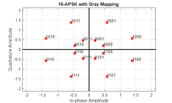
Create a custom-coded symbol mapping vector. This custom mapping happens to be another Gray-coded mapping.
cmap = [0;1;9;8;12;13;5;4;2;3;11;10;14;15;7;6];
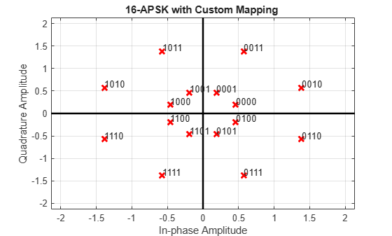
Apply APSK modulation with a custom-coded symbol mapping. Plot the constellation using binary input to highlight that the custom mapping defines different Gray-coded symbol mapping.
z = apskmod(xBit,M,radii, ...
    SymbolMapping=cmap, ...
    PlotConstellation=true, ...
    InputType='bit');
Demodulate MIL-STD-188-110C Specific 64-QAM Signal
Demodulate a 64-QAM signal that was modulated as specified in MIL-STD-188-110C. Compute hard decision bit output and verify that the output matches the input.
Set the modulation order and generate random bit data.
M = 64;
numBitsPerSym = log2(M);
x = randi([0 1],1000*numBitsPerSym,1);
Modulate the data. Use name-value pairs to specify bit input data and to plot the constellation.
txSig = mil188qammod(x,M,InputType='bit',PlotConstellation=true);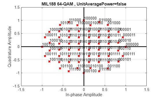
Demodulate the received signal. Compare the demodulated data to the original data.
z = mil188qamdemod(txSig,M,OutputType='bit');
isequal(z,x)
ans = logical
1
Demodulate Noisy 16-APSK Signal Using Simulink
Apply 16-APSK modulation to a signal of random data. Pass the modulated signal through an AWGN channel. Demodulate the noisy 16-APSK signal. The example reports bit error rate (BER) and symbol error rate (SER) at two SNR settings.
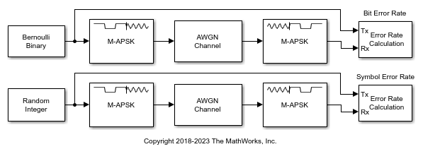
The slex_16apsk_mod model passes a 16-APSK modulated signal through an AWGN channel, demodulates the signal and then computes the error rate statistics. The upper workflow computes the BER and the lower workflow computes the SER. Some block parameters get set by using workspace variables initialized in the PreLoadFcn callback function loads simulation variables into the workspace. For more information, see Model Callbacks (Simulink).
Run the model with the AWGN channel blocks set to EbN0 = 6 dB and display the computed BER and SER. The AWGN Channel block in the lower workflow converts the EbN0 setting to an EsN0 setting. The results are saved to the workspace variables BERVec and SERVec in 1-by-3 row vectors. The first element contains the error rate.
With EbN0 set to  6.00 dB, BER: 0.070
With EsN0 set to 12.02 dB, SER: 0.160
Change the EbN0 of the AWGN channel block to 10 dB. Run the model, display the computed BER and SER, and observe the decrease in error rate.
With EbN0 set to 10.00 dB, BER: 0.016
With EsN0 set to 16.02 dB, SER: 0.051
See Also
Functions
Objects
Blocks
- Raised Cosine Transmit Filter | Raised Cosine Receive Filter | M-APSK Modulator Baseband | M-APSK Demodulator Baseband | MIL-188 QAM Modulator Baseband | MIL-188 QAM Demodulator Baseband