R =
Results for
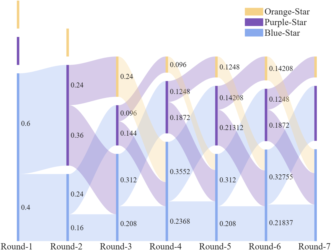
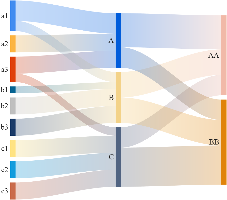
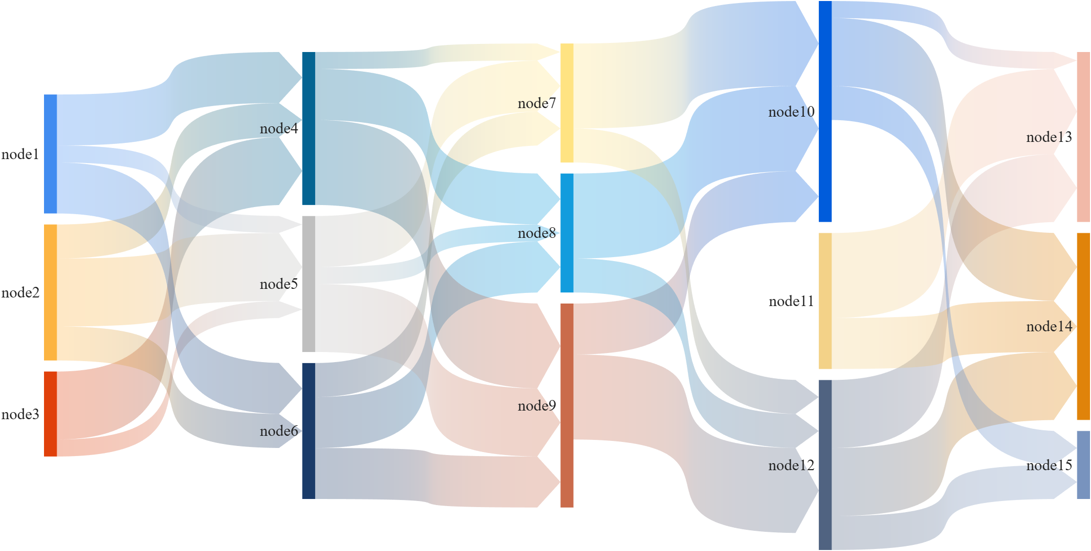
This is a brief introduction and recommendation of a Sankey diagram plotting tool:
Basic usage - links
links={'a1','A',1.2;'a2','A',1;'a1','B',.6;'a3','A',1; 'a3','C',0.5;
'b1','B',.4; 'b2','B',1;'b3','B',1; 'c1','C',1;
'c2','C',1; 'c3','C',1;'A','AA',2; 'A','BB',1.2;
'B','BB',1.5; 'B','AA',1.5; 'C','BB',2.3; 'C','AA',1.2};
% 创建桑基图对象(Create a Sankey diagram object)
SK=SSankey(links(:,1),links(:,2),links(:,3));
% 开始绘图(Start drawing)
SK.draw()
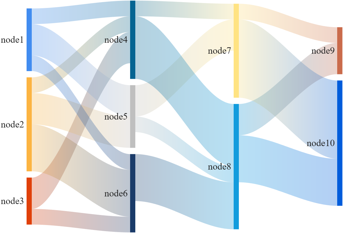
Basic usage - adjMat
% Define inter-layer adjacency matrices
% 定义层间邻接矩阵
A12 = [1,2,1; 1,2,3; 2,0,1];
A23 = [1,4; 2,1; 0,3];
A34 = [1,5; 2,3];
% Assemble global block matrix (main diagonal = zero, super-diagonal = A12, A23, A34)
% 组装全局分块矩阵(主对角线为零,上对角线为 A12, A23, A34)
adjMat = mergeAdjMat({A12, A23, A34});
SK = SSankey([],[],[], 'AdjMat',adjMat);
SK.draw()
Further usage examples can be found in the demos included in the compressed package:
I've been confused trying to write (or have an AI write) the .m (Live) text format from scratch for various reasons using .mlx format exported with the IDE as .m (old) and .m (LIve). Of course, one problem is the .m and .m (Live) files have the same name,causing confusion and requiring renaming, but repeatedly, after sussing out and following all conventions for headings and latex etc in .m (LIve), my .m (Live) files would not open as .mlx in the IDE. I think I've found the answer by trial and error and comparison and don't know it is documented. Add at the end
%[appendix]{"version":"1.0"} %--- %[metadata:view] % data: {"layout":"inline"} %---
This seems to trigger the IDE to recognize this is a .m (Live). Woohoo! This is a LOT easier than writing .mlx zip packages from scratch.
Have you ever wondered what it takes to send live audio from one computer to another? While we use apps like Discord and Zoom every day, the core technology behind real-time voice communication is a fascinating blend of audio processing and networking. Building a simple walkie-talkie is a perfect project for demystifying these concepts, and you can do it all within the powerful environment of MATLAB.
This article will guide you through creating a functional, real-time, push-to-talk walkie-talkie. We won't be building a replacement for a commercial radio, but we will create a powerful educational tool that demonstrates the fundamentals of digital signal processing and network communication.
The Purpose: Why Build This?
The goal isn't just to talk to a colleague across the office; it's to learn by doing. By building this project, you will:
Understand Audio I/O: Learn how MATLAB interacts with your computer’s microphone and speakers.
Grasp Network Communication: See how to send data packets over a local network using the UDP protocol.
Solve Real-Time Challenges: Confront and solve issues like latency, choppy audio, and continuous data streaming.
The Core Components
Our walkie-talkie will consist of two main scripts:
Sender.m: This script will run on the transmitting computer. It listens to the microphone when a key is pressed, sending the audio data in small chunks over the network.
Receiver.m: This script runs on the receiving computer. It continuously listens for incoming data packets and plays them through the speakers as they arrive.
Step 1: Getting Audio In and Out
Before we touch networking, let's make sure we can capture and play audio. MATLAB's built-in audiorecorder and audioplayer objects make this simple.
Problem Encountered: How do you even access the microphone?
Solution: The audiorecorder object gives us straightforward control.
code
% --- Test Audio Capture and Playback ---
Fs = 8000; % Sample rate in Hz
nBits = 16; % Number of bits per sample
nChannels = 1; % Mono audio
% Create a recorder object
recObj = audiorecorder(Fs, nBits, nChannels);
disp('Start speaking for 3 seconds.');
recordblocking(recObj, 3); % Record for 3 seconds
disp('End of Recording.');
% Get the audio data
audioData = getaudiodata(recObj);
% Play it back
playObj = audioplayer(audioData, Fs);
play(playObj);
Running this script confirms that your microphone and speakers are correctly configured and accessible by MATLAB.
Step 2: Sending Voice Over the Network
Now, we need to send the audioData to another computer. For real-time applications like this, the UDP (User Datagram Protocol) is the ideal choice. It’s a "fire-and-forget" protocol that prioritizes speed over perfect reliability. Losing a tiny packet of audio is better than waiting for it to be re-sent, which would cause noticeable delays (latency).
Problem Encountered: How do you send data continuously without overwhelming the network or the receiver?
Solution: We'll send the audio in small, manageable chunks inside a loop. We need to create a UDP Port object to handle the communication.
Here's the basic structure for the Sender.m script:
code
% --- Sender.m ---
% Define network parameters
remoteIP = '192.168.1.101'; % <--- CHANGE THIS to the receiver's IP
remotePort = 3000;
localPort = 3001;
% Create UDP Port object
udpSender = udpport("LocalPort", localPort, "EnablePortSharing", true);
% Configure audio recorder
Fs = 8000;
nBits = 16;
nChannels = 1;
recObj = audiorecorder(Fs, nBits, nChannels);
disp('Press any key to start transmitting. Press Ctrl+C to stop.');
pause; % Wait for user to press a key
% Start the Push-to-Talk loop
disp('Transmitting... (Hold Ctrl+C to exit)');
while true
recordblocking(recObj, 0.1); % Record a 0.1-second chunk
audioChunk = getaudiodata(recObj);
% Send the audio chunk over UDP
write(udpSender, audioChunk, "double", remoteIP, remotePort);
end
And here is the corresponding Receiver.m script:
code
Matlab
% --- Receiver.m ---
% Define network parameters
localPort = 3000;
% Create UDP Port object
udpReceiver = udpport("LocalPort", localPort, "EnablePortSharing", true, "Timeout", 30);
% Configure audio player
Fs = 8000;
playerObj = audioplayer(zeros(Fs*0.1, 1), Fs); % Pre-buffer
disp('Listening for incoming audio...');
% Start the listening loop
while true
% Wait for and receive data
[audioChunk, ~, ~] = read(udpReceiver, Fs*0.1, "double");
if ~isempty(audioChunk)
% Play the received audio chunk
play(playerObj, audioChunk);
else
disp('No data received. Still listening...');
end
end
Step 3: Solving Real-World Hurdles
Running the code above might work, but you'll quickly notice some issues.
Problem 1: Choppy Audio and High Latency
The audio might sound robotic or delayed. This is because of the buffer size and the processing time. Sending tiny chunks frequently can cause overhead, while sending large chunks causes delay.
Solution: The key is to find a balance.
Tune the Chunk Size: The 0.1 second chunk size in the sender (recordblocking(recObj, 0.1)) is a good starting point. Experiment with values between 0.05 and 0.2. Smaller values reduce latency but increase network traffic.
Use a Buffered Player: Instead of creating a new audioplayer for every chunk, we create one at the start and feed it new data. Our receiver code already does this, which is more efficient.
Problem 2: No Real "Push-to-Talk"
Our sender script starts transmitting and doesn't stop. A real walkie-talkie only transmits when a button is held down.
Solution: Simulating this in a script requires a more advanced technique, ideally using a MATLAB App Designer GUI. However, we can create a simple command-window version using a figure's KeyPressFcn.
Here is an improved concept for the Sender that simulates radio push-to-talk, e.g. https://www.retevis.com/blog/ptt-push-to-talk-walkie-talkies-guide
% --- Advanced_Sender.m ---
function PushToTalkSender()
% -- Configuration --
remoteIP = '192.168.1.101'; % <--- CHANGE THIS
remotePort = 3000;
localPort = 3001;
Fs = 8000;
% -- Setup --
udpSender = udpport("LocalPort", localPort);
recObj = audiorecorder(Fs, 16, 1);
% -- GUI for key press detection --
fig = uifigure('Name', 'Push-to-Talk (Hold ''t'')', 'Position', [100 100 300 100]);
fig.KeyPressFcn = @KeyPress;
fig.KeyReleaseFcn = @KeyRelease;
isTransmitting = false; % Flag to control transmission
disp('Focus on the figure window. Hold the ''t'' key to transmit.');
% --- Main Loop ---
while ishandle(fig)
if isTransmitting
% Non-blocking record and send would be ideal,
% but for simplicity we use short blocking chunks.
recordblocking(recObj, 0.1);
audioChunk = getaudiodata(recObj);
write(udpSender, audioChunk, "double", remoteIP, remotePort);
disp('Transmitting...');
else
pause(0.1); % Don't burn CPU when idle
end
drawnow; % Update figure window
end
% --- Callback Functions ---
function KeyPress(~, event)
if strcmp(event.Key, 't')
isTransmitting = true;
end
end
function KeyRelease(~, event)
if strcmp(event.Key, 't')
isTransmitting = false;
disp('Transmission stopped.');
end
end
end
Conclusion and Next Steps
You've now built the foundation of a real-time voice communication tool in MATLAB! You've learned how to capture audio, send it over a network using UDP, and handle some of the fundamental challenges of real-time streaming.
This project is the perfect starting point for more advanced explorations:
Build a Full GUI: Use App Designer to create a user-friendly interface with a proper push-to-talk radio button.
Implement Noise Reduction: Apply a filter (e.g., a simple low-pass or a more advanced spectral subtraction algorithm) to the audioChunk before sending it.
Add Channels: Modify the code to use different UDP ports, allowing users to select a "channel" to talk on.
In a previous discussion,
we looked at a variety of infallible tests for primality, but all of them were too slow to be viable for large numbers. In fact, all of the methods discussed there will fail miserably for even moderately large numbers, those with just a few dozen decimal digits. That does not even begin to push into the realm of large numbers. In turn, that forces us into a different realm of tests - tests which are usually and even almost always correct, but can sometimes incorrectly predict primality.
In this discussion, I will be trying to convince you that the Fermat test for primality can be a quite good test when the number is sufficiently large. Except of course, when it is really bad. Even so, the Fermat test for primality is both a useful tool as well as a necessary underpinning for several other better tests.
The Fermat test for primality relies on Fermat's little theorem, a perhaps under-appreciated tool. Even the name implies it is of little interest. I'm not taking about the famous last theorem, only proven in recent years, but his little theorem.
If you want to look over some nice ways to prove the little theorem, take a read in this link:
I will readily admit that long ago, when I learned about the little theorem in a nearly forgotten class, I thought it was interesting, but why would I care? Not until I learned more mathematics and saw Fermat’s little theorem appearing in different places did I begin to appreciate it. Fermat tells us that, IF P is a prime, AND w is co-prime with P (so the two are relatively prime, sharing no common factors except 1), then it must be true that
mod(w^(P-1),P) == 1
Try it out. Does it work? Be careful though as too large of an exponent will cause problems in double precision, and that is not difficult to do. As a test case that will not overwhelm doubles, note that 13 is prime, and 3 shares no common factors with 13, so we satisfy the requirements for Fermat's little theorem.
mod(3^12,13)
We can even verify that any co-prime of 13 will yield the same result.
mod((1:12).^12,13)
Indeed it worked, suggesting what we knew all along, that 13 is prime. The little Fermat test for primality of the number P uses a converse form of Fermat's little theorem, thus given a co-prime number w known as the witness, is that if
mod(w^(P-1),P)==1
then we have evidence that P is indeed prime. This is not conclusive evidence, but still it is evidence. It is not conclusive because the converse of a true statement is not always true.
The analogy I like here is if we lived in a universe where all crows are black. (I'll ask you to pretend this is true. In fact, some crows have a mutation, making them essentially albino crows. For the purposes of this thought experiment, pretend this cannot happen.) Now, suppose I show you a picture of a bird which happens to be black. Do you know the bird to be a crow? Of course not, as the bird may be a raven, or a redwing blackbird (until you see the splash of red on the wing), a common grackle, a European starling in summer plumage, a condor, etc. But having seen black plumage, it is now more likely the bird is indeed a crow. I would call this a moderately weak evidentiary test for crow-ness.
Little Fermat may seem to be of little value when testing for primality for two reasons. First, computing the remainder would seem to be highly CPU intensive for large P. In the example above, I had only to compute 3^12=531441, which is not that large. But for numbers with many thousands or millions of digits, directly raising even a number as small as 2 to that power will overwhelm any computer. Secondly, if we do that computation, little Fermat does not conclusively prove P to be prime.
Our savior in one respect is the powermod tool. And that helps greatly, since we can compute the remainder in a reasonable time. A powermod call is quite fast even for huge powers. (I won't get into how powermod works here, since that alone is probably worth a discussion. I could though, if I see some interest because there are some very pretty variations of the powermod algorithm. I hope to show you one of them when I discuss the Fibonacci test for primality in a future post.) Trying the little Fermat test using powermod on a number with 1207 decimal digits, I’ll first do a time check.
P = 4000*sym(2)^3999 - 1;
timeit(@() powermod(2,P-1,P))
As you can see, powermod really is pretty fast. Compared to an isprime test on that number it would show a significant difference.
I have said before that little Fermat is not a conclusive test. In fact, a good trick is to perform a second little Fermat test, using a different witness. If the second test also indicates primality, then we have additional evidence that P is in fact prime.
w = [2 3]; % Two parallel witnesses
powermod(w,P-1,P)
This value for P is indeed prime, and little Fermat suggests it is, doubly suggestive in that test since I actually performed two parallel tests. Here however, we need to understand when it will fail, and how often it will fail.
If we perform a little Fermat test for primality, we will never see false negatives, that is, if any test with any witness ever indicates a number is composite, then it is certainly composite. (The contrapositive of a true statement is always true.) The alternate class of failure is the false positive, where little Fermat indicates a number is prime when it was actually composite.
If P is composite, and w co-prime with P, we call P a Fermat pseudo-prime for the witness w if we see a remainder of 1 when P was in fact composite. When that happens, the witness (w) is called a Fermat liar for the primality of P. (A list of some Fermat pseudo-primes where 2 is a Fermat liar can be found in sequence A001567 of the OEIS.)
In the case of 4000*2^3999-1, I claimed the number to be in fact prime, and it was identified so (as PROBABLY prime by little Fermat. Next, consider another number from that same family. I’ll perform three parallel tests on it, with witnesses 2, 3, and 5. This will suggest the value of doing parallel tests on a number to reduce the failure rate from little Fermat.
P2 = 1024*sym(2)^1023 - 1;
w = [2; 3; 5];
gcd(w,P2)
F2 = powermod(w,P2-1,P2)
logical(F2 == 1)
As you can see, P2 is co-prime with all of 2, 3 and 5, but 2 is a Fermat liar, whilst 3 and 5 are Fermat truth tellers, identifying P2 as certainly composite. So the little Fermat test can definitely fail for SOME witnesses, since we see a disagreement. However, an interesting fact about P2 above is it is also a Mersenne number with prime exponent, thus it can be written as 2^1033-1, where 1033 is prime. I can go into more detail about this case later, but we can show that 2 is always a Fermat liar for composite Mersenne numbers when the exponent is itself prime. I’ll try to leave more detail on this matter in a future discussion, or perhaps a comment.
Next, consider the composite integer 51=3*17. As the product of two primes, it is clearly not itself prime.
P51 = 51;
w0 = 2:P51-2;
w = w0(gcd(w0,P51) == 1)
Note that I did not include 1 or 50 in that set, since 1 raised to any power is 1, and 50 is congruent to -1, mod 51. -1 raised to any even power is also always 1, and 51-1 is an even number. And so when we are working modulo 51, both 1 and 50 are not useful witnesses in terms of the little Fermat test.
R = powermod(w,P-1,P)
w(R == 1)
This teaches us that when 51 is tested for primality using the little Fermat test, there are 2 distinct witnesses w (16 and 35) we could have chosen which would have been Fermat liars, but all 28 other potential co-prime witnesses would have been truth tellers, accurately showing 51 to be composite. Proportionally, little Fermat will have been correct roughly 93% of the time, since only 2 of these 30 possible tests returned a false positive. (I’ll add that for any modulus P, if w<P is not co-prime with the modulus, then the computation mod(w^(P-1),P) will always return a non-unit result, and therefore we can theoretically use any integer w from the set 2:P-2 as a witness. However if w is co-prime with P then P is clearly not prime, and the entire problem becomes a little less interesting. As such, I will only consider co-prime witnesses for this discussion.) Regardless, that would make the little Fermat test for P=51 even more often correct, since it returns the correct result of composite for 46 out of the 48 possible witnesses 2:49. Does this mean Little Fermat is indeed the basis for a good test to rely on to learn if a number is prime? Well, yes. And no.
Little Fermat forms a very good test most of the time, but reliance is a strong word. This means we need to explore the little Fermat test in more depth, focusing on Fermat liars and the case of false positives. To offer some appreciation of the false positive rate, offline, I have tested all composite integers between 4 and 10000, for all their possible co-prime witnesses.
load FermatLiarsData
In that .mat file, I've saved three vectors, X, witnessCount, and liarCount. X is there just to use for plotting purposes and is NaN for all non-composite entries.
whos X witnessCount liarCount
The vector witnessCount is the number of valid witnesses for the corresponding number in X. Corresponding to that is the vector liarCount, which is the number of Fermat liars I found for each composite in X.
How many Fermat test useful witnesses are there for any integer X? This is just 2 less than the number of coprimes of X. The number of coprimes is given by the Euler totient function, commonly called phi(X). (I’ll be going into more depth on the totient in the next chapter of this series, because the Euler totient is a crucial part of understanding how all of this works.)
The witness count is phi(X)-2. Why subtract 2? 1 can never be a witness, but 1 is technically coprime to everything. The same applies to X-1 (which is congruent to -1 mod X.) As such, there are phi(X)-2 coprimes to consider. (I've posted a function called totient on the FEX, but it is easily computed if you know the factorization of X. Or for small numbers, you can just use GCD to identify all co-primes, and count them.)
plot(X,witnessCount,'.')
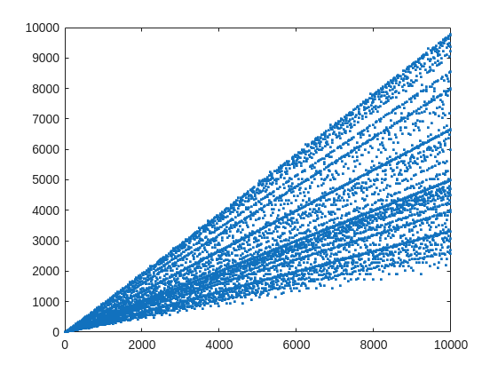
From that plot, you can learn a few interesting things. (As a mathematician, this is what I love the most, thus to look at whay may be the simplest, most boring plot, and try to find something of value, something I had never thought of before.) For example, we know that when X is prime, then everything from the set 2:X-2 is a valid witness. So the upper boundary on that plot will be the line y==x. As well, there are a few numbers where the order of the set of witnesses will be close to the maximum possible. For example, 961=31*31, has 928 valid witnesses. That makes some sense, as 961 is the square of a prime (31), so we know 961 is divisible only by 31. Only multiples of 31 will not be coprime with 961.
But how about the lower boundary? The least number of valid witnesses will always come from highly composite numbers, because they will share common factors with almost everything. For example 30 = 2*3*5, or 210=2*3*5*7.
witnessCount([30 210 420])
A good discussion about the lower bound for that plot can be found here:
What really matters to us though, is the fraction of the useful witnesses for a little Fermat test that yield a false positive.
plot(X,liarCount./witnessCount,'b.')
Cind = liarCount == witnessCount;
hold on
plot(X(Cind),1,'ro')
ylabel('Liar fraction')
xlabel('X')
title('Fermat pseudo-prime strength')
hold off
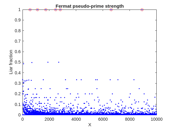
A look at this plot shows seven circles in red, corresponding to X from the list {561, 1105, 1729, 2465, 2821, 6601, 8911} which are collectively known as Carmichael numbers. These are numbers where all witnesses return a false positive. Carmichael numbers are themselves fairly rare. You can find a list of them as sequence A002997 in the OEIS. And for those of you who have never wandered around the OEIS, please take this opportunity to do so now. The OEIS stands for Online Encyclopedia of Integer Sequences. It contains a wealth of interesting knowledge about integers and integer sequences.)
There are a few other interesting numbers we can find in that plot, like 91 and 703, where roughly 50% of the valid witnesses yield false positives. Of the complete set, which numbers did return at least a 25% false positive rate for primality? These numbers would be known as strong pseudo-primes for the little Fermat test, because they are pseudo-primes for at least 25% of the potential witnesses. These strong pseudo-primes have some interesting similarities to the Carmichael numbers. (My next post will go into more depth on Carmichael numbers and strong pseudo-primes. At the moment, I am merely interested in looking at the how often the little Fermat test fails overall.)
find(liarCount./witnessCount> 0.25)
You should notice the spacing between successive strong Fermat pseudo-primes is growing slowly, with a spacing of roughly 800 on average in the vicinity of 10000. If I step out beyond by a factor of 10, the next strong Fermat pseudo-primes after 1e5 are {101101, 104653, 107185, 109061, 111361, 114589, 115921 126217, 126673}, so that average spacing is definitely growing.
Given that set, now we can look at the prime factorizations of each of those strong pseudo-primes. Can we learn something about them?
arrayfun(@factor,find(liarCount./witnessCount> 0.25),'UniformOutput',false)
Perhaps the most glaring thing I see in that set of factors is almost all of those strong Fermat pseudo-primes are square free. That is, in that list, only 45=3*3*5 had any replicated factor at all. That property of being square free is something we will see is necessary to be a Carmichael number, but it also suggests that a simple roughness test applied in advance would have eliminated almost all of those strong pseudo-primes as obviously not prime, even at a very low level of roughness.
In fact, for most composite integers, most witnesses do indeed return a negative, indicating the number is not prime, and therefore composite. Little Fermat does not commonly tell falsehoods, even though it can do so.
semilogy(X,movmedian(liarCount./witnessCount,20,'omitnan'),'b-')
title('False positive fraction for composites')
yline(0.0003,'r')

We can learn from this last plot that as the number to be tested grows large, the median false positive rate for little Fermat, even for X as low as only 10000, is roughly 0.0003. (It continues to decrease for larger X too. In fact, I’ve read that when X is on the order of 2^256, the relative fraction of Fermat liars is on the order of 1 in 1e12, and it continues to decrease as X grows in magnitude. In my eyes, that seems pretty good for an imperfect test. Not perfect, but not bad when paired with roughness and perhaps a second little Fermat test using a different witness, and we will start to see tests which bear a higher degree of strength.)
I’ll stop at this point in this post because the post is getting lengthy. In my next post, I’d like to visit some questions about what are Carmichael numbers, about whether some witnesses are better than others, and if there are any numbers which lack any Fermat liars. However, in order to dive more deeply, I will need to explain how/why/when the little Fermat test works, and what causes Fermat liars. Stay tuned, because this starts to get interesting.
Over the past few days I noticed a minor change on the MATLAB File Exchange:
For a FEX repository, if you click the 'Files' tab you now get a file-tree–style online manager layout with an 'Open in new tab' hyperlink near the top-left. This is very useful:
If you want to share that specific page externally (e.g., on GitHub), you can simply copy that hyperlink. For .mlx files it provides a perfect preview. I'd love to hear your thoughts.
EXAMPLE:
🤗🤗🤗
I recently created a short 5-minute video covering 10 tips for students learning MATLAB. I hope this helps!
You may have come across code that looks like that in some languages:
stubFor(get(urlPathEqualTo("/quotes"))
.withHeader("Accept", equalTo("application/json"))
.withQueryParam("s", equalTo(monitoredStock))
.willReturn(aResponse())
.withStatus(200)
.withHeader("Content-Type", "application/json")
.withBody("{\\"symbol\\": \\"XYZ\\", \\"bid\\": 20.2, " + "\\"ask\\": 20.6}")))
That’s Java. Even if you can’t fully decipher it, you can get a rough idea of what it is supposed to do, build a rather complex API query.
Or you may be familiar with the following similar and frequent syntax in Python:
import seaborn as sns
sns.load_dataset('tips').sample(10, random_state=42).groupby('day').mean()
Here’s is how it works: multiple method calls are linked together in a single statement, spanning over one or several lines, usually because each method returns the same object or another object that supports further calls.
That technique is called method chaining and is popular in Object-Oriented Programming.
A few years ago, I looked for a way to write code like that in MATLAB too. And the answer is that it can be done in MATLAB as well, whevener you write your own class!
Implementing a method that can be chained is simply a matter of writing a method that returns the object itself.
In this article, I would like to show how to do it and what we can gain from such a syntax.
Example
A few years ago, I first sought how to implement that technique for a simulation launcher that had lots of parameters (far too many):
lauchSimulation(2014:2020, true, 'template', 'TmplProd', 'Priority', '+1', 'Memory', '+6000')
As you can see, that function takes 2 required inputs, and 3 named parameters (whose names aren’t even consistent, with ‘Priority’ and ‘Memory’ starting with an uppercase letter when ‘template’ doesn’t).
(The original function had many more parameters that I omit for the sake of brevity. You may also know of such functions in your own code that take a dozen parameters which you can remember the exact order.)
I thought it would be nice to replace that with:
SimulationLauncher() ...
.onYears(2014:2020) ...
.onDistributedCluster() ... % = equivalent of the previous "true"
.withTemplate('TmplProd') ...
.withPriority('+1') ...
.withReservedMemory('+6000') ...
.launch();
The first 6 lines create an object of class SimulationLauncher, calls several methods on that object to set the parameters, and lastly the method launch() is called, when all desired parameters have been set.
To make it cleared, the syntax previously shown could also be rewritten as:
launcher = SimulationLauncher();
launcher = launcher.onYears(2014:2020);
launcher = launcher.onDistributedCluster();
launcher = launcher.withTemplate('TmplProd');
launcher = launcher.withPriority('+1');
launcher = launcher.withReservedMemory('+6000');
launcher.launch();
Before we dive into how to implement that code, let’s examine the advantages and drawbacks of that syntax.
Benefits and drawbacks
Because I have extended the chained methods over several lines, it makes it easier to comment out or uncomment any one desired option, should the need arise. Furthermore, we need not bother any more with the order in which we set the parameters, whereas the usual syntax required that we memorize or check the documentation carefully for the order of the inputs.
More generally, chaining methods has the following benefits and a few drawbacks:
Benefits:
- Conciseness: Code becomes shorter and easier to write, by reducing visual noise compared to repeating the object name.
- Readability: Chained methods create a fluent, human-readable structure that makes intent clear.
- Reduced Temporary Variables: There's no need to create intermediary variables, as the methods directly operate on the object.
Drawbacks:
- Debugging Difficulty: If one method in a chain fails, it can be harder to isolate the issue. It effectively prevents setting breakpoints, inspecting intermediate values, and identifying which method failed.
- Readability Issues: Overly long and dense method chains can become hard to follow, reducing clarity.
- Side Effects: Methods that modify objects in place can lead to unintended side effects when used in long chains.
Implementation
In the SimulationLauncher class, the method lauch performs the main operation, while the other methods just serve as parameter setters. They take the object as input and return the object itself, after modifying it, so that other methods can be chained.
classdef SimulationLauncher
properties (GetAccess = private, SetAccess = private)
years_
isDistributed_ = false;
template_ = 'TestTemplate';
priority_ = '+2';
memory_ = '+5000';
end
methods
function varargout = launch(obj)
% perform whatever needs to be launched
% using the values of the properties stored in the object:
% obj.years_
% obj.template_
% etc.
end
function obj = onYears(obj, years)
assert(isnumeric(years))
obj.years_ = years;
end
function obj = onDistributedCluster(obj)
obj.isDistributed_ = true;
end
function obj = withTemplate(obj, template)
obj.template_ = template;
end
function obj = withPriority(obj, priority)
obj.priority_ = priority;
end
function obj = withMemory( obj, memory)
obj.memory_ = memory;
end
end
end
As you can see, each method can be in charge of verifying the correctness of its input, independantly. And what they do is just store the value of parameter inside the object. The class can define default values in the properties block.
You can configure different launchers from the same initial object, such as:
launcher = SimulationLauncher();
launcher = launcher.onYears(2014:2020);
launcher1 = launcher ...
.onDistributedCluster() ...
.withReservedMemory('+6000');
launcher2 = launcher ...
.withTemplate('TmplProd') ...
.withPriority('+1') ...
.withReservedMemory('+7000');
If you call the same method several times, only the last recorded value of the parameter will be taken into acount:
launcher = SimulationLauncher();
launcher = launcher ...
.withReservedMemory('+6000') ...
.onDistributedCluster() ...
.onYears(2014:2020) ...
.withReservedMemory('+7000') ...
.withReservedMemory('+8000');
% The value of "memory" will be '+8000'.
If the logic is still not clear to you, I advise you play a bit with the debugger to better understand what’s going on!
Conclusion
I love how the method chaining technique hides the minute detail that we don’t want to bother with when trying to understand what a piece of code does.
I hope this simple example has shown you how to apply it to write and organise your code in a more readable and convenient way.
Let me know if you have other questions, comments or suggestions. I may post other examples of that technique for other useful uses that I encountered in my experience.
If you use tables extensively to perform data analysis, you may at some point have wanted to add new functionalities suited to your specific applications. One straightforward idea is to create a new class that subclasses the built-in table class. You would then benefit from all inherited existing methods.
One workaround is to create a new class that wraps a table as a Property, and re-implement all the methods that you need and are already defined for table. The is not too difficult, except for the subsref method, for which I’ll provide the code below.
Class definition
Defining a wrapper of the table class is quite straightforward. In this example, I call the class “Report” because that is what I intend to use the class for, to compute and store reports. The constructor just takes a table as input:
classdef Rapport
methods
function obj = Report(t)
if isa(t, 'Report')
obj = t;
else
obj.t_ = t;
end
end
end
properties (GetAccess = private, SetAccess = private)
t_ table = table();
end
end
I designed the constructor so that it converts a table into a Report object, but also so that if we accidentally provide it with a Report object instead of a table, it will not generate an error.
Reproducing the behaviour of the table class
Implementing the existing methods of the table class for the Report class if pretty easy in most cases.
I made use of a method called “table” in order to be able to get the data back in table format instead of a Report, instead of accessing the property t_ of the object. That method can also be useful whenever you wish to use the methods or functions already existing for tables (such as writetable, rowfun, groupsummary…).
classdef Rapport
...
methods
function t = table(obj)
t = obj.t_;
end
function r = eq(obj1,obj2)
r = isequaln(table(obj1), table(obj2));
end
function ind = size(obj, varargin)
ind = size(table(obj), varargin{:});
end
function ind = height(obj, varargin)
ind = height(table(obj), varargin{:});
end
function ind = width(obj, varargin)
ind = width(table(obj), varargin{:});
end
function ind = end(A,k,n)
% ind = end(A.t_,k,n);
sz = size(table(A));
if k < n
ind = sz(k);
else
ind = prod(sz(k:end));
end
end
end
end
In the case of horzcat (same principle for vertcat), it is just a matter of converting back and forth between the table and Report classes:
classdef Rapport
...
methods
function r = horzcat(obj1,varargin)
listT = cell(1, nargin);
listT{1} = table(obj1);
for k = 1:numel(varargin)
kth = varargin{k};
if isa(kth, 'Report')
listT{k+1} = table(kth);
elseif isa(kth, 'table')
listT{k+1} = kth;
else
error('Input must be a table or a Report');
end
end
res = horzcat(listT{:});
r = Report(res);
end
end
end
Adding a new method
The plus operator already exists for the table class and works when the table contains all numeric values. It sums columns as long as the tables have the same length.
Something I think would be nice would be to be able to write t1 + t2, and that would perform an outerjoin operation between the tables and any sizes having similar indexing columns.
That would be so concise, and that's what we’re going to implement for the Report class as an example. That is called “plus operator overloading”. Of course, you could imagine that the “+” operator is used to compute something else, for example adding columns together with regard to the keys index. That depends on your needs.
Here’s a unittest example:
classdef ReportTest < matlab.unittest.TestCase
methods (Test)
function testPlusOperatorOverload(testCase)
t1 = array2table( ...
{ 'Smith', 'Male' ...
; 'JACKSON', 'Male' ...
; 'Williams', 'Female' ...
} , 'VariableNames', {'LastName' 'Gender'} ...
);
t2 = array2table( ...
{ 'Smith', 13 ...
; 'Williams', 6 ...
; 'JACKSON', 4 ...
}, 'VariableNames', {'LastName' 'Age'} ...
);
r1 = Report(t1);
r2 = Report(t2);
tRes = r1 + r2;
tExpected = Report( array2table( ...
{ 'JACKSON' , 'Male', 4 ...
; 'Smith' , 'Male', 13 ...
; 'Williams', 'Female', 6 ...
} , 'VariableNames', {'LastName' 'Gender' 'Age'} ...
) );
testCase.verifyEqual(tRes, tExpected);
end
end
end
And here’s how I’d implement the plus operator in the Report class definition, so that it also works if I add a table and a Report:
classdef Rapport
...
methods
function r = plus(obj1,obj2)
table1 = table(obj1);
table2 = table(obj2);
result = outerjoin(table1, table2 ...
, 'Type', 'full', 'MergeKeys', true);
r = reportingits.dom.Rapport(result);
end
end
end
The case of the subsref method
If we wish to access the elements of an instance the same way we would with regular tables, whether with parentheses, curly braces or directly with the name of the column, we need to implement the subsref and subsasgn methods. The second one, subsasgn is pretty easy, but subsref is a bit tricky, because we need to detect whether we’re directing towards existing methods or not.
Here’s the code:
classdef Rapport
...
methods
function A = subsasgn(A,S,B)
A.t_ = subsasgn(A.t_,S,B);
end
function B = subsref(A,S)
isTableMethod = @(m) ismember(m, methods('table'));
isReportMethod = @(m) ismember(m, methods('Report'));
switch true
case strcmp(S(1).type, '.') && isReportMethod(S(1).subs)
methodName = S(1).subs;
B = A.(methodName)(S(2).subs{:});
if numel(S) > 2
B = subsref(B, S(3:end));
end
case strcmp(S(1).type, '.') && isTableMethod (S(1).subs)
methodName = S(1).subs;
if ~isReportMethod(methodName)
error('The method "%s" needs to be implemented!', methodName)
end
otherwise
B = subsref(table(A),S(1));
if istable(B)
B = Report(B);
end
if numel(S) > 1
B = subsref(B, S(2:end));
end
end
end
end
end
Conclusion
I believe that the table class is Sealed because is case new methods are introduced in MATLAB in the future, the subclass might not be compatible if we created any or generate unexpected complexity.
The table class is a really powerful feature.
I hope this example has shown you how it is possible to extend the use of tables by adding new functionalities and maybe given you some ideas to simplify some usages. I’ve only happened to find it useful in very restricted cases, but was still happy to be able to do so.
In case you need to add other methods of the table class, you can see the list simply by calling methods(’table’).
Feel free to share your thoughts or any questions you might have! Maybe you’ll decide that doing so is a bad idea in the end and opt for another solution.

It’s exciting to dive into a new dataset full of unfamiliar variables but it can also be overwhelming if you’re not sure where to start. Recently, I discovered some new interactive features in MATLAB live scripts that make it much easier to get an overview of your data. With just a few clicks, you can display sparklines and summary statistics using table variables, sort and filter variables, and even have MATLAB generate the corresponding code for reproducibility.
The Graphics and App Building blog published an article that walks through these features showing how to explore, clean, and analyze data—all without writing any code.
If you’re interested in streamlining your exploratory data analysis or want to see what’s new in live scripts, you might find it helpful:
If you’ve tried these features or have your own tips for quick data exploration in MATLAB, I’d love to hear your thoughts!
I just learned you can access MATLAB Online from the following shortcut in your web browser: https://matlab.new
Thanks @Yann Debray
From his recent blog post: pip & uv in MATLAB Online » Artificial Intelligence - MATLAB & Simulink
What if you had no isprime utility to rely on in MATLAB? How would you identify a number as prime? An easy answer might be something tricky, like that in simpleIsPrime0.
simpleIsPrime0 = @(N) ismember(N,primes(N));
But I’ll also disallow the use of primes here, as it does not really test to see if a number is prime. As well, it would seem horribly inefficient, generating a possibly huge list of primes, merely to learn something about the last member of the list.
Looking for a more serious test for primality, I’ve already shown how to lighten the load by a bit using roughness, to sometimes identify numbers as composite and therefore not prime.
https://www.mathworks.com/matlabcentral/discussions/tips/879745-primes-and-rough-numbers-basic-ideas
But to actually learn if some number is prime, we must do a little more. Yes, this is a common homework problem assigned to students, something we have seen many times on Answers. It can be approached in many ways too, so it is worth looking at the problem in some depth.
The definition of a prime number is a natural number greater than 1, which has only two factors, thus 1 and itself. That makes a simple test for primality of the number N easy. We just try dividing the number by every integer greater than 1, and not exceeding N-1. If any of those trial divides leaves a zero remainder, then N cannot be prime. And of course we can use mod or rem instead of an explicit divide, so we need not worry about floating point trash, as long as the numbers being tested are not too large.
simpleIsPrime1 = @(N) all(mod(N,2:N-1) ~= 0);
Of course, simpleIsPrime1 is not a good code, in the sense that it fails to check if N is an integer, or if N is less than or equal to 1. It is not vectorized, and it has no documentation at all. But it does the job well enough for one simple line of code. There is some virtue in simplicity after all, and it is certainly easy to read. But sometimes, I wish a function handle could include some help comments too! A feature request might be in the offing.
simpleIsPrime1(9931)
simpleIsPrime1(9932)
simpleIsPrime1 works quite nicely, and seems pretty fast. What could be wrong? At some point, the student is given a more difficult problem, to identify if a significantly larger integer is prime. simpleIsPrime1 will then cause a computer to grind to a distressing halt if given a sufficiently large number to test. Or it might even error out, when too large a vector of numbers was generated to test against. For example, I don't think you want to test a number of the order of 2^64 using simpleIsPrime1, as performing on the order of 2^64 divides will be highly time consuming.
uint64(2)^63-25
Is it prime? I’ve not tested it to learn if it is, and simpleIsPrime1 is not the tool to perform that test anyway.
A student might realize the largest possible integer factors of some number N are the numbers N/2 and N itself. But, if N/2 is a factor, then so is 2, and some thought would suggest it is sufficient to test only for factors that do not exceed sqrt(N). This is because if a is a divisor of N, then so is b=N/a. If one of them is larger than sqrt(N), then the other must be smaller. That could lead us to an improved scheme in simpleIsPrime2.
simpleIsPrime2 = @(N) all(mod(N,2:sqrt(N)));
For an integer of the size 2^64, now you only need to perform roughly 2^32 trial divides. Maybe we might consider the subtle improvement found in simpleIsPrime3, which avoids trial divides by the even integers greater than 2.
simpleIsPrime3 = @(N) (N == 2) || (mod(N,2) && all(mod(N,3:2:sqrt(N))));
simpleIsPrime3 needs only an approximate maximum of 2^31 trial divides even for numbers as large as uint64 can represent. While that is large, it is still generally doable on the computers we have today, even if it might be slow.
Sadly, my goals are higher than even the rather lofty limit given by UINT64 numbers. The problem of course is that a trial divide scheme, despite being 100% accurate in its assessment of primality, is a time hog. Even an O(sqrt(N)) scheme is far too slow for numbers with thousands or millions of digits. And even for a number as “small” as 1e100, a direct set of trial divides by all primes less than sqrt(1e100) would still be practically impossible, as there are roughly n/log(n) primes that do not exceed n. For an integer on the order of 1e50,
1e50/log(1e50)
It is practically impossible to perform that many divides on any computer we can make today. Can we do better? Is there some more efficient test for primality? For example, we could write a simple sieve of Eratosthenes to check each prime found not exceeding sqrt(N).
function [TF,SmallPrime] = simpleIsPrime4(N)
% simpleIsPrime3 - Sieve of Eratosthenes to identify if N is prime
% [TF,SmallPrime] = simpleIsPrime3(N)
%
% Returns true if N is prime, as well as the smallest prime factor
% of N when N is composite. If N is prime, then SmallPrime will be N.
Nroot = ceil(sqrt(N)); % ceil caters for floating point issues with the sqrt
TF = true;
SieveList = true(1,Nroot+1); SieveList(1) = false;
SmallPrime = 2;
while TF
% Find the "next" true element in SieveList
while (SmallPrime <= Nroot+1) && ~SieveList(SmallPrime)
SmallPrime = SmallPrime + 1;
end
% When we drop out of this loop, we have found the next
% small prime to check to see if it divides N, OR, we
% have gone past sqrt(N)
if SmallPrime > Nroot
% this is the case where we have now looked at all
% primes not exceeding sqrt(N), and have found none
% that divide N. This is where we will drop out to
% identify N as prime. TF is already true, so we need
% not set TF.
SmallPrime = N;
return
else
if mod(N,SmallPrime) == 0
% smallPrime does divide N, so we are done
TF = false;
return
end
% update SieveList
SieveList(SmallPrime:SmallPrime:Nroot) = false;
end
end
end
simpleIsPrime4 does indeed work reasonably well, though it is sometimes a little slower than is simpleIsPrime3, and everything is hugely faster than simpleIsPrime1.
timeit(@() simpleIsPrime1(111111111))
timeit(@() simpleIsPrime2(111111111))
timeit(@() simpleIsPrime3(111111111))
timeit(@() simpleIsPrime4(111111111))
All of those times will slow to a crawl for much larger numbers of course. And while I might find a way to subtly improve upon these codes, any improvement will be marginal in the end if I try to use any such direct approach to primality. We must look in a different direction completely to find serious gains.
At this point, I want to distinguish between two distinct classes of tests for primality of some large number. One class of test is what I might call an absolute or infallible test, one that is perfectly reliable. These are tests where if X is identified as prime/composite then we can trust the result absolutely. The tests I showed in the form of simpleIsPrime1, simpleIsPrime2, simpleIsPrime3 and aimpleIsprime4, were all 100% accurate, thus they fall into the class of infallible tests.
The second general class of test for primality is what I will call an evidentiary test. Such a test provides evidence, possibly quite strong evidence, that the given number is prime, but in some cases, it might be mistaken. I've already offered a basic example of a weak evidentiary test for primality in the form of roughness. All primes are maximally rough. And therefore, if you can identify X as being rough to some extent, this provides evidence that X is also prime, and the depth of the roughness test influences the strength of the evidence for primality. While this is generally a fairly weak test, it is a test nevertheless, and a good exclusionary test, a good way to avoid more sophisticated but time consuming tests.
These evidentiary tests all have the property that if they do identify X as being composite, then they are always correct. In the context of roughness, if X is not sufficiently rough, then X is also not prime. On the other side of the coin, if you can show X is at least (sqrt(X)+1)-rough, then it is positively prime. (I say this to suggest that some evidentiary tests for primality can be turned into truth telling tests, but that may take more effort than you can afford.) The problem is of course that is literally impossible to verify that degree of roughness for numbers with many thousands of digits.
In my next post, I'll look at the Fermat test for primality, based on Fermat's little theorem.
I saw an interesting problem on a reddit math forum today. The question was to find a number (x) as close as possible to r=3.6, but the requirement is that both x and 1/x be representable in a finite number of decimal places.
The problem of course is that 3.6 = 18/5. And the problem with 18/5 has an inverse 5/18, which will not have a finite representation in decimal form.
In order for a number and its inverse to both be representable in a finite number of decimal places (using base 10) we must have it be of the form 2^p*5^q, where p and q are integer, but may be either positive or negative. If that is not clear to you intuitively, suppose we have a form
2^p*5^-q
where p and q are both positive. All you need do is multiply that number by 10^q. All this does is shift the decimal point since you are just myltiplying by powers of 10. But now the result is
2^(p+q)
and that is clearly an integer, so the original number could be represented using a finite number of digits as a decimal. The same general idea would apply if p was negative, or if both of them were negative exponents.
Now, to return to the problem at hand... We can obviously adjust the number r to be 20/5 = 4, or 16/5 = 3.2. In both cases, since the fraction is now of the desired form, we are happy. But neither of them is really close to 3.6. My goal will be to find a better approximation, but hopefully, I can avoid a horrendous amount of trial and error. It would seem the trick might be to take logs, to get us closer to a solution. That is, suppose I take logs, to the base 2?
log2(3.6)
I used log2 here because that makes the problem a little simpler, since log2(2^p)=p. Therefore we want to find a pair of integers (p,q) such that
log2(3.6) + delta = p + log2(5)*q
where delta is as close to zero as possible. Thus delta is the error in our approximation to 3.6. And since we are working in logs, delta can be viewed as a proportional error term. Again, p and q may be any integers, either positive or negative. The two cases we have seen already have (p,q) = (2,0), and (4,-1).
Do you see the general idea? The line we have is of the form
log2(3.6) = p + log2(5)*q
it represents a line in the (p,q) plane, and we want to find a point on the integer lattice (p,q) where the line passes as closely as possible.
[Xl,Yl] = meshgrid([-10:10]);
plot(Xl,Yl,'k.')
hold on
fimplicit(@(p,q) -log2(3.6) + p + log2(5)*q,[-10,10,-10,10],'g-')
plot([2 4],[0,-1],'ro')
hold off
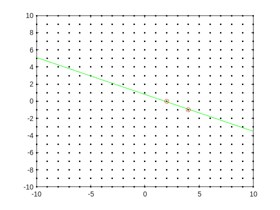
Now, some might think in terms of orthogonal distance to the line, but really, we want the vertical distance to be minimized. Again, minimize abs(delta) in the equation:
log2(3.6) + delta = p + log2(5)*q
where p and q are integer.
Can we do that using MATLAB? The skill about about mathematics often lies in formulating a word problem, and then turning the word problem into a problem of mathematics that we know how to solve. We are almost there now. I next want to formulate this into a problem that intlinprog can solve. The problem at first is intlinprog cannot handle absolute value constraints. And the trick there is to employ slack variables, a terribly useful tool to emply on this class of problem.
Rewrite delta as:
delta = Dpos - Dneg
where Dpos and Dneg are real variables, but both are constrained to be positive.
prob = optimproblem;
p = optimvar('p',lower = -50,upper = 50,type = 'integer');
q = optimvar('q',lower = -50,upper = 50,type = 'integer');
Dpos = optimvar('Dpos',lower = 0);
Dneg = optimvar('Dneg',lower = 0);
Our goal for the ILP solver will be to minimize Dpos + Dneg now. But since they must both be positive, it solves the min absolute value objective. One of them will always be zero.
r = 3.6;
prob.Constraints = log2(r) + Dpos - Dneg == p + log2(5)*q;
prob.Objective = Dpos + Dneg;
The solve is now a simple one. I'll tell it to use intlinprog, even though it would probably figure that out by itself. (Note: if I do not tell solve which solver to use, it does use intlinprog. But it also finds the correct solution when I told it to use GA offline.)
solve(prob,solver = 'intlinprog')
The solution it finds within the bounds of +/- 50 for both p and q seems pretty good. Note that Dpos and Dneg are pretty close to zero.
2^39*5^-16
and while 3.6028979... seems like nothing special, in fact, it is of the form we want.
R = sym(2)^39*sym(5)^-16
vpa(R,100)
vpa(1/R,100)
both of those numbers are exact. If I wanted to find a better approximation to 3.6, all I need do is extend the bounds on p and q. And we can use the same solution approch for any floating point number.
Since R2024b, a Levenberg–Marquardt solver (TrainingOptionsLM) was introduced. The built‑in function trainnet now accepts training options via the trainingOptions function (https://www.mathworks.com/help/deeplearning/ref/trainingoptions.html#bu59f0q-2) and supports the LM algorithm. I have been curious how to use it in deep learning, and the official documentation has not provided a concrete usage example so far. Below I give a simple example to illustrate how to use this LM algorithm to optimize a small number of learnable parameters.
For example, consider the nonlinear function:
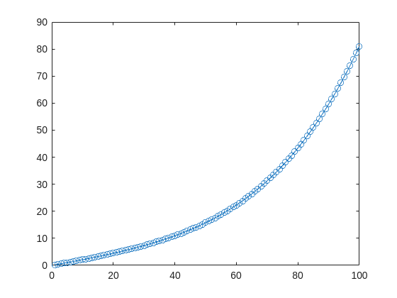
y_hat = @(a,t) a(1)*(t/100) + a(2)*(t/100).^2 + a(3)*(t/100).^3 + a(4)*(t/100).^4;
It represents a curve. Given 100 matching points (t → y_hat), we want to use least squares to estimate the four parameters a1–a4.
t = (1:100)';
y_hat = @(a,t)a(1)*(t/100) + a(2)*(t/100).^2 + a(3)*(t/100).^3 + a(4)*(t/100).^4;
x_true = [ 20 ; 10 ; 1 ; 50 ];
y_true = y_hat(x_true,t);
plot(t,y_true,'o-')
- Using the traditional lsqcurvefit-wrapped "Levenberg–Marquardt" algorithm:
x_guess = [ 5 ; 2 ; 0.2 ; -10 ];
options = optimoptions("lsqcurvefit",Algorithm="levenberg-marquardt",MaxFunctionEvaluations=800);
[x,resnorm,residual,exitflag] = lsqcurvefit(y_hat,x_guess,t,y_true,-50*ones(4,1),60*ones(4,1),options);
x,resnorm,exitflag
- Using the deep-learning-wrapped "Levenberg–Marquardt" algorithm:
options = trainingOptions("lm", ...
InitialDampingFactor=0.002, ...
MaxDampingFactor=1e9, ...
DampingIncreaseFactor=12, ...
DampingDecreaseFactor=0.2,...
GradientTolerance=1e-6, ...
StepTolerance=1e-6,...
Plots="training-progress");
numFeatures = 1;
layers = [featureInputLayer(numFeatures,'Name','input')
fitCurveLayer(Name='fitCurve')];
net = dlnetwork(layers);
XData = dlarray(t);
YData = dlarray(y_true);
netTrained = trainnet(XData,YData,net,"mse",options);
netTrained.Layers(2)
classdef fitCurveLayer < nnet.layer.Layer ...
& nnet.layer.Acceleratable
% Example custom SReLU layer.
properties (Learnable)
% Layer learnable parameters
a1
a2
a3
a4
end
methods
function layer = fitCurveLayer(args)
arguments
args.Name = "lm_fit";
end
% Set layer name.
layer.Name = args.Name;
% Set layer description.
layer.Description = "fit curve layer";
end
function layer = initialize(layer,~)
% layer = initialize(layer,layout) initializes the layer
% learnable parameters using the specified input layout.
if isempty(layer.a1)
layer.a1 = rand();
end
if isempty(layer.a2)
layer.a2 = rand();
end
if isempty(layer.a3)
layer.a3 = rand();
end
if isempty(layer.a4)
layer.a4 = rand();
end
end
function Y = predict(layer, X)
% Y = predict(layer, X) forwards the input data X through the
% layer and outputs the result Y.
% Y = layer.a1.*exp(-X./layer.a2) + layer.a3.*X.*exp(-X./layer.a4);
Y = layer.a1*(X/100) + layer.a2*(X/100).^2 + layer.a3*(X/100).^3 + layer.a4*(X/100).^4;
end
end
end
The network is very simple — only the fitCurveLayer defines the learnable parameters a1–a4. I observed that the output values are very close to those from lsqcurvefit.
Function Syntax Design Conundrum
As a MATLAB enthusiast, I particularly enjoy Steve Eddins' blog and the cool things he explores. MATLAB's new argument blocks are great, but there's one frustrating limitation that Steve outlined beautifully in his blog post "Function Syntax Design Conundrum": cases where an argument should accept both enumerated values AND other data types.
Steve points out this could be done using the input parser, but I prefer having tab completions and I'm not a fan of maintaining function signature JSON files for all my functions.
Personal Context on Enumerations
To be clear: I honestly don't like enumerations in any way, shape, or form. One reason is how awkward they are. I've long suspected they're simply predefined constructor calls with a set argument, and I think that's all but confirmed here. This explains why I've had to fight the enumeration system when trying to take arguments of many types and normalize them to enumerated members, or have numeric values displayed as enumerated members without being recast to the superclass every operation.
The Discovery
While playing around extensively with metadata for another project, I realized (and I'm entirely unsure why it took so long) that the properties of a metaclass object are just, in many cases, the attributes of the classdef. In this realization, I found a solution to Steve's and my problem.
To be clear: I'm not in love with this solution. I would much prefer a better approach for allowing variable sets of membership validation for arguments. But as it stands, we don't have that, so here's an interesting, if incredibly hacky, solution.
If you call struct() on a metaclass object to view its hidden properties, you'll notice that in addition to the public "Enumeration" property, there's a hidden "Enumerable" property. They're both logicals, which implies they're likely functionally distinct. I was curious about that distinction and hoped to find some functionality by intentionally manipulating these values - and I did, solving the exact problem Steve mentions.
The Problem Statement
We have a function with an argument that should allow "dual" input types: enumerated values (Steve's example uses days of the week, mine uses the "all" option available in various dimension-operating functions) AND integers. We want tab completion for the enumerated values while still accepting the numeric inputs.
A Solution for Tab-Completion Supported Arguments
Rather than spoil Steve's blog post, let me use my own example: implementing a none() function. The definition is simple enough tf = ~any(A, dim); but when we wrap this in another function, we lose the tab-completion that any() provides for the dim argument (which gives you "all"). There's no great way to implement this as a function author currently - at least, that's well documented.
So here's my solution:
%% Example Function Implementation
% This is a simple implementation of the DimensionArgument class for implementing dual type inputs that allow enumerated tab-completion.
function tf = none(A, dim)
arguments(Input)
A logical;
dim DimensionArgument = DimensionArgument(A, true);
end
% Simple example (notice the use of uplus to unwrap the hidden property)
tf = ~any(A, +dim);
end
I like this approach because the additional work required to implement it, once the enumeration class is initialized, is minimal. Here are examples of function calls, note that the behavior parallels that of the MATLAB native-style tab-completion:
%% Test Data
% Simple logical array for testing
A = randi([0, 1], [3, 5], "logical");
%% Example function calls
tf = none(A, "all"); % This is the tab-completion it's 1:1 with MATLABs behavior
tf = none(A, [1, 2]); % We can still use valid arguments (validated in the constructor)
tf = none(A); % Showcase of the constructors use as a default argument generator
How It Works
What makes this work is the previously mentioned Enumeration attribute. By setting Enumeration = false while still declaring an enumeration block in the classdef file, we get the suggested members as auto-complete suggestions. As I hinted at, the value of enumerations (if you don't subclass a builtin and define values with the someMember (1) syntax) are simply arguments to constructor calls.
We also get full control over the storage and handling of the class, which means we lose the implicit storage that enumerations normally provide and are responsible for doing so ourselves - but I much prefer this. We can implement internal validation logic to ensure values that aren't in the enumerated set still comply with our constraints, and store the input (whether the enumerated member or alternative type) in an internal property.
As seen in the example class below, this maintains a convenient interface for both the function caller and author the only particuarly verbose portion is the conversion methods... Which if your willing to double down on the uplus unwrapping context can be avoided. What I have personally done is overload the uplus function to return the input (or perform the identity property) this allowss for the uplus to be used universally to unwrap inputs and for those that cant, and dont have a uplus definition, the value itself is just returned:
classdef(Enumeration = false) DimensionArgument % < matlab.mixin.internal.MatrixDisplay
%DimensionArgument Enumeration class to provide auto-complete on functions needing the dimension type seen in all()
% Enumerations are just macros to make constructor calls with a known set of arguments. Declaring the 'all'
% enumeration member means this class can be set as the type for an input and the auto-completion for the given
% argument will show the enumeration members, allowing tab-completion. Declaring the Enumeration attribute of
% the class as false gives us control over the constructor and internal implementation. As such we can use it
% to validate the numeric inputs, in the event the 'all' option was not used, and return an object that will
% then work in place of valid dimension argument options.
%% Enumeration members
% These are the auto-complete options you'd like to make available for the function signature for a given
% argument.
enumeration(Description="Enumerated value for the dimension argument.")
all
end
%% Properties
% The internal property allows the constructor's input to be stored; this ensures that the value is store and
% that the output of the constructor has the class type so that the validation passes.
% (Constructors must return the an object of the class they're a constructor for)
properties(Hidden, Description="Storage of the constructor input for later use.")
Data = [];
end
%% Constructor method
% By the magic of declaring (Enumeration = false) in our class def arguments we get full control over the
% constructor implementation.
%
% The second argument in this specific instance is to enable the argument's default value to be set in the
% arguments block itself as opposed to doing so in the function body... I like this better but if you didn't
% you could just as easily keep the constructor simple.
methods
function obj = DimensionArgument(A, Adim)
%DimensionArgument Initialize the dimension argument.
arguments
% This will be the enumeration member name from auto-completed entries, or the raw user input if not
% used.
A = [];
% A flag that indicates to create the value using different logic, in this case the first non-singleton
% dimension, because this matches the behavior of functions like, all(), sum() prod(), etc.
Adim (1, 1) logical = false;
end
if(Adim)
% Allows default initialization from an input to match the aforemention function's behavior
obj.Data = firstNonscalarDim(A);
else
% As a convenience for this style of implementation we can validate the input to ensure that since we're
% suppose to be an enumeration, the input is valid
DimensionArgument.mustBeValidMember(A);
% Store the input in a hidden property since declaring ~Enumeration means we are responsible for storing
% it.
obj.Data = A;
end
end
end
%% Conversion methods
% Applies conversion to the data property so that implicit casting of functions works. Unfortunately most of
% the MathWorks defined functions use a different system than that employed by the arguments block, which
% defers to the class defined converter methods... Which is why uplus (+obj) has been defined to unwrap the
% data for ease of use.
methods
function obj = uplus(obj)
obj = obj.Data;
end
function str = char(obj)
str = char(obj.Data);
end
function str = cellstr(obj)
str = cellstr(obj.Data);
end
function str = string(obj)
str = string(obj.Data);
end
function A = double(obj)
A = double(obj.Data);
end
function A = int8(obj)
A = int8(obj.Data);
end
function A = int16(obj)
A = int16(obj.Data);
end
function A = int32(obj)
A = int32(obj.Data);
end
function A = int64(obj)
A = int64(obj.Data);
end
end
%% Validation methods
% These utility methods are for input validation
methods(Static, Access = private)
function tf = isValidMember(obj)
%isValidMember Checks that the input is a valid dimension argument.
tf = (istext(obj) && all(obj == "all", "all")) || (isnumeric(obj) && all(isint(obj) & obj > 0, "all"));
end
function mustBeValidMember(obj)
%mustBeValidMember Validates that the input is a valid dimension argument for the dim/dimVec arguments.
if(~DimensionArgument.isValidMember(obj))
exception("JB:DimensionArgument:InvalidInput", "Input must be an integer value or the term 'all'.")
end
end
end
%% Convenient data display passthrough
methods
function disp(obj, name)
arguments
obj DimensionArgument
name string {mustBeScalarOrEmpty} = [];
end
% Dispatch internal data's display implementation
display(obj.Data, char(name));
end
end
end
In the event you'd actually play with theres here are the function definitions for some of the utility functions I used in them, including my exception would be a pain so i wont, these cases wont use it any...
% Far from my definition isint() but is consistent with mustBeInteger() for real numbers but will suffice for the example
function tf = isint(A)
arguments
A {mustBeNumeric(A)};
end
tf = floor(A) == A
end
% Sort of the same but its fine
function dim = firstNonscalarDim(A)
arguments
A
end
dim = [find(size(A) > 1, 1), 0];
dim(1) = dim(1);
end
Hello MATLAB Central, this is my first article.
My name is Yann. And I love MATLAB.
I also love HTTP (i know, weird fetish)
So i started a conversation with ChatGPT about it:
gitclone('https://github.com/yanndebray/HTTP-with-MATLAB');
cd('HTTP-with-MATLAB')
http_with_MATLAB
I'm not sure that this platform is intended to clone repos from github, but i figured I'd paste this shortcut in case you want to try out my live script http_with_MATLAB.m
A lot of what i program lately relies on external web services (either for fetching data, or calling LLMs).
So I wrote a small tutorial of the 7 or so things I feel like I need to remember when making HTTP requests in MATLAB.
Let me know what you think
Did you know that function double with string vector input significantly outperforms str2double with the same input:
x = rand(1,50000);
t = string(x);
tic; str2double(t); toc
tic; I1 = str2double(t); toc
tic; I2 = double(t); toc
isequal(I1,I2)
Recently I needed to parse numbers from text. I automatically tried to use str2double. However, profiling revealed that str2double was the main bottleneck in my code. Than I realized that there is a new note (since R2024a) in the documentation of str2double:
"Calling string and then double is recommended over str2double because it provides greater flexibility and allows vectorization. For additional information, see Alternative Functionality."
t = turtle(); % Start a turtle
t.forward(100); % Move forward by 100
t.backward(100); % Move backward by 100
t.left(90); % Turn left by 90 degrees
t.right(90); % Tur right by 90 degrees
t.goto(100, 100); % Move to (100, 100)
t.turnto(90); % Turn to 90 degrees, i.e. north
t.speed(1000); % Set turtle speed as 1000 (default: 500)
t.pen_up(); % Pen up. Turtle leaves no trace.
t.pen_down(); % Pen down. Turtle leaves a trace again.
t.color('b'); % Change line color to 'b'
t.begin_fill(FaceColor, EdgeColor, FaceAlpha); % Start filling
t.end_fill(); % End filling
t.change_icon('person.png'); % Change the icon to 'person.png'
t.clear(); % Clear the Axes
classdef turtle < handle
properties (GetAccess = public, SetAccess = private)
x = 0
y = 0
q = 0
end
properties (SetAccess = public)
speed (1, 1) double = 500
end
properties (GetAccess = private)
speed_reg = 100
n_steps = 20
ax
l
ht
im
is_pen_up = false
is_filling = false
fill_color
fill_alpha
end
methods
function obj = turtle()
figure(Name='MATurtle', NumberTitle='off')
obj.ax = axes(box="on");
hold on,
obj.ht = hgtransform();
icon = flipud(imread('turtle.png'));
obj.im = imagesc(obj.ht, icon, ...
XData=[-30, 30], YData=[-30, 30], ...
AlphaData=(255 - double(rgb2gray(icon)))/255);
obj.l = plot(obj.x, obj.y, 'k');
obj.ax.XLim = [-500, 500];
obj.ax.YLim = [-500, 500];
obj.ax.DataAspectRatio = [1, 1, 1];
obj.ax.Toolbar.Visible = 'off';
disableDefaultInteractivity(obj.ax);
end
function home(obj)
obj.x = 0;
obj.y = 0;
obj.ht.Matrix = eye(4);
end
function forward(obj, dist)
obj.step(dist);
end
function backward(obj, dist)
obj.step(-dist)
end
function step(obj, delta)
if numel(delta) == 1
delta = delta*[cosd(obj.q), sind(obj.q)];
end
if obj.is_filling
obj.fill(delta);
else
obj.move(delta);
end
end
function goto(obj, x, y)
dx = x - obj.x;
dy = y - obj.y;
obj.turnto(rad2deg(atan2(dy, dx)));
obj.step([dx, dy]);
end
function left(obj, q)
obj.turn(q);
end
function right(obj, q)
obj.turn(-q);
end
function turnto(obj, q)
obj.turn(obj.wrap_angle(q - obj.q, -180));
end
function pen_up(obj)
if obj.is_filling
warning('not available while filling')
return
end
obj.is_pen_up = true;
end
function pen_down(obj, go)
if obj.is_pen_up
if nargin == 1
obj.l(end+1) = plot(obj.x, obj.y, Color=obj.l(end).Color);
else
obj.l(end+1) = go;
end
uistack(obj.ht, 'top')
end
obj.is_pen_up = false;
end
function color(obj, line_color)
if obj.is_filling
warning('not available while filling')
return
end
obj.pen_up();
obj.pen_down(plot(obj.x, obj.y, Color=line_color));
end
function begin_fill(obj, FaceColor, EdgeColor, FaceAlpha)
arguments
obj
FaceColor = [.6, .9, .6];
EdgeColor = [0 0.4470 0.7410];
FaceAlpha = 1;
end
if obj.is_filling
warning('already filling')
return
end
obj.fill_color = FaceColor;
obj.fill_alpha = FaceAlpha;
obj.pen_up();
obj.pen_down(patch(obj.x, obj.y, [1, 1, 1], ...
EdgeColor=EdgeColor, FaceAlpha=0));
obj.is_filling = true;
end
function end_fill(obj)
if ~obj.is_filling
warning('not filling now')
return
end
obj.l(end).FaceColor = obj.fill_color;
obj.l(end).FaceAlpha = obj.fill_alpha;
obj.is_filling = false;
end
function change_icon(obj, filename)
icon = flipud(imread(filename));
obj.im.CData = icon;
obj.im.AlphaData = (255 - double(rgb2gray(icon)))/255;
end
function clear(obj)
obj.x = 0;
obj.y = 0;
delete(obj.ax.Children(2:end));
obj.l = plot(0, 0, 'k');
obj.ht.Matrix = eye(4);
end
end
methods (Access = private)
function animated_step(obj, delta, q, initFcn, updateFcn)
arguments
obj
delta
q
initFcn = @() []
updateFcn = @(~, ~) []
end
dx = delta(1)/obj.n_steps;
dy = delta(2)/obj.n_steps;
dq = q/obj.n_steps;
pause_duration = norm(delta)/obj.speed/obj.speed_reg;
initFcn();
for i = 1:obj.n_steps
updateFcn(dx, dy);
obj.ht.Matrix = makehgtform(...
translate=[obj.x + dx*i, obj.y + dy*i, 0], ...
zrotate=deg2rad(obj.q + dq*i));
pause(pause_duration)
drawnow limitrate
end
obj.x = obj.x + delta(1);
obj.y = obj.y + delta(2);
end
function obj = turn(obj, q)
obj.animated_step([0, 0], q);
obj.q = obj.wrap_angle(obj.q + q, 0);
end
function move(obj, delta)
initFcn = @() [];
updateFcn = @(dx, dy) [];
if ~obj.is_pen_up
initFcn = @() initializeLine();
updateFcn = @(dx, dy) obj.update_end_point(obj.l(end), dx, dy);
end
function initializeLine()
obj.l(end).XData(end+1) = obj.l(end).XData(end);
obj.l(end).YData(end+1) = obj.l(end).YData(end);
end
obj.animated_step(delta, 0, initFcn, updateFcn);
end
function obj = fill(obj, delta)
initFcn = @() initializePatch();
updateFcn = @(dx, dy) obj.update_end_point(obj.l(end), dx, dy);
function initializePatch()
obj.l(end).Vertices(end+1, :) = obj.l(end).Vertices(end, :);
obj.l(end).Faces = 1:size(obj.l(end).Vertices, 1);
end
obj.animated_step(delta, 0, initFcn, updateFcn);
end
end
methods (Static, Access = private)
function update_end_point(l, dx, dy)
l.XData(end) = l.XData(end) + dx;
l.YData(end) = l.YData(end) + dy;
end
function q = wrap_angle(q, min_angle)
q = mod(q - min_angle, 360) + min_angle;
end
end
end
I would like to zoom directly on the selected region when using  on my image created with image or imagesc. First of all, I would recommend using image or imagesc and not imshow for this case, see comparison here: Differences between imshow() and image()? However when zooming Stretch-to-Fill behavior happens and I don't want that. Try range zoom to image generated by this code:
fig = uifigure;
ax = uiaxes(fig);
im = imread("peppers.png");
h = imagesc(im,"Parent",ax);
axis(ax,'tight', 'off')
I can fix that with manualy setting data aspect ratio:
daspect(ax,[1 1 1])
However, I need this code to run automatically after zooming. So I create zoom object and ActionPostCallback which is called everytime after I zoom, see zoom - ActionPostCallback.
z = zoom(ax);
z.ActionPostCallback = @(fig,ax) daspect(ax.Axes,[1 1 1]);
If you need, you can also create ActionPreCallback which is called everytime before I zoom, see zoom - ActionPreCallback.
z.ActionPreCallback = @(fig,ax) daspect(ax.Axes,'auto');
Code written and run in R2025a.
I am thrilled python interoperability now seems to work for me with my APPLE M1 MacBookPro and MATLAB V2025a. The available instructions are still, shall we say, cryptic. Here is a summary of my interaction with GPT 4o to get this to work.
===========================================================
MATLAB R2025a + Python (Astropy) Integration on Apple Silicon (M1/M2/M3 Macs)
===========================================================
Author: D. Carlsmith, documented with ChatGPT
Last updated: July 2025
This guide provides full instructions, gotchas, and workarounds to run Python 3.10 with MATLAB R2025a (Apple Silicon/macOS) using native ARM64 Python and calling modules like Astropy, Numpy, etc. from within MATLAB.
===========================================================
Overview
===========================================================
- MATLAB R2025a on Apple Silicon (M1/M2/M3) runs as "maca64" (native ARM64).
- To call Python from MATLAB, the Python interpreter must match that architecture (ARM64).
- Using Intel Python (x86_64) with native MATLAB WILL NOT WORK.
- The cleanest solution: use Miniforge3 (Conda-forge's lightweight ARM64 distribution).
===========================================================
1. Install Miniforge3 (ARM64-native Conda)
===========================================================
In Terminal, run:
curl -LO https://github.com/conda-forge/miniforge/releases/latest/download/Miniforge3-MacOSX-arm64.sh
bash Miniforge3-MacOSX-arm64.sh
Follow prompts:
- Press ENTER to scroll through license.
- Type "yes" when asked to accept the license.
- Press ENTER to accept the default install location: ~/miniforge3
- When asked:
Do you wish to update your shell profile to automatically initialize conda? [yes|no]
Type: yes
===========================================================
2. Restart Terminal and Create a Python Environment for MATLAB
===========================================================
Run the following:
conda create -n matlab python=3.10 astropy numpy -y
conda activate matlab
Verify the Python path:
which python
Expected output:
/Users/YOURNAME/miniforge3/envs/matlab/bin/python
===========================================================
3. Verify Python + Astropy From Terminal
===========================================================
Run:
python -c "import astropy; print(astropy.__version__)"
Expected output:
6.x.x (or similar)
===========================================================
4. Configure MATLAB to Use This Python
===========================================================
In MATLAB R2025a (Apple Silicon):
clear classes
pyenv('Version', '/Users/YOURNAME/miniforge3/envs/matlab/bin/python')
py.sys.version
You should see the Python version printed (e.g. 3.10.18). No error means it's working.
===========================================================
5. Gotchas and Their Solutions
===========================================================
❌ Error: Python API functions are not available
→ Cause: Wrong architecture or broken .dylib
→ Fix: Use Miniforge ARM64 Python. DO NOT use Intel Anaconda.
❌ Error: Invalid text character (↑ points at __version__)
→ Cause: MATLAB can’t parse double underscores typed or pasted
→ Fix: Use: py.getattr(module, '__version__')
❌ Error: Unrecognized method 'separation' or 'sec'
→ Cause: MATLAB can't reflect dynamic Python methods
→ Fix: Use: py.getattr(obj, 'method')(args)
===========================================================
6. Run Full Verification in MATLAB
===========================================================
Paste this into MATLAB:
% Set environment
clear classes
pyenv('Version', '/Users/YOURNAME/miniforge3/envs/matlab/bin/python');
% Import modules
coords = py.importlib.import_module('astropy.coordinates');
time_mod = py.importlib.import_module('astropy.time');
table_mod = py.importlib.import_module('astropy.table');
% Astropy version
ver = char(py.getattr(py.importlib.import_module('astropy'), '__version__'));
disp(['Astropy version: ', ver]);
% SkyCoord angular separation
c1 = coords.SkyCoord('10h21m00s', '+41d12m00s', pyargs('frame', 'icrs'));
c2 = coords.SkyCoord('10h22m00s', '+41d15m00s', pyargs('frame', 'icrs'));
sep_fn = py.getattr(c1, 'separation');
sep = sep_fn(c2);
arcsec = double(sep.to('arcsec').value);
fprintf('Angular separation = %.3f arcsec\n', arcsec);
% Time difference in seconds
Time = time_mod.Time;
t1 = Time('2025-01-01T00:00:00', pyargs('format','isot','scale','utc'));
t2 = Time('2025-01-02T00:00:00', pyargs('format','isot','scale','utc'));
dt = py.getattr(t2, '__sub__')(t1);
seconds = double(py.getattr(dt, 'sec'));
fprintf('Time difference = %.0f seconds\n', seconds);
% Astropy table display
tbl = table_mod.Table(pyargs('names', {'a','b'}, 'dtype', {'int','float'}));
tbl.add_row({1, 2.5});
tbl.add_row({2, 3.7});
disp(tbl);
===========================================================
7. Optional: Automatically Configure Python in startup.m
===========================================================
To avoid calling pyenv() every time, edit your MATLAB startup:
edit startup.m
Add:
try
pyenv('Version', '/Users/YOURNAME/miniforge3/envs/matlab/bin/python');
catch
warning("Python already loaded.");
end
===========================================================
8. Final Notes
===========================================================
- This setup avoids all architecture mismatches.
- It uses a clean, minimal ARM64 Python that integrates seamlessly with MATLAB.
- Do not mix Anaconda (Intel) with Apple Silicon MATLAB.
- Use py.getattr for any Python attribute containing underscores or that MATLAB can't resolve.
You can now run NumPy, Astropy, Pandas, Astroquery, Matplotlib, and more directly from MATLAB.
===========================================================