imodwt
Inverse maximal overlap discrete wavelet transform
Syntax
Description
xrec = imodwt(w)w. By default, imodwt
assumes that you obtained w using the 'sym4'
wavelet with periodic boundary handling. If you do not modify the coefficients,
xrec is a perfect reconstruction of the signal.
xrec = imodwt(___,'reflection')'reflection', imodwt assumes
that the length of the original signal length is one half the number
of columns in the input coefficient matrix. By default, imodwt assumes
periodic signal extension at the boundary.
You must enter the entire character vector 'reflection'. If you
added a wavelet named 'reflection' using the wavelet manager, you
must rename that wavelet prior to using this option. 'reflection'
may be placed in any position in the input argument list after
x.
Examples
Obtain the MODWT of an ECG signal and demonstrate perfect reconstruction.
Load the ECG signal data and obtain the MODWT.
load wecg;Obtain the MODWT and the Inverse MODWT.
w = modwt(wecg);
xrec = imodwt(w);
Use the L-infinity norm to show that the difference between the original signal and the reconstruction is extremely small. The largest absolute difference between the original signal and the reconstruction is on the order of , which demonstrates perfect reconstruction.
norm(abs(xrec'-wecg),Inf)
ans =
2.3255e-12
Obtain the MODWT of Deutsche Mark-U.S. Dollar exchange rate data and demonstrate perfect reconstruction.
Load the Deutsche Mark-U.S. Dollar exchange rate data.
load DM_USD;Obtain the MODWT and the Inverse MODWT using the 'db2' wavelet.
wdm = modwt(DM_USD,'db2');
xrec = imodwt(wdm,'db2');
Use the L-infinity norm to show that the difference between the original signal and the reconstruction is extremely small. The largest absolute difference between the original signal and the reconstruction is on the order of , which demonstrates perfect reconstruction.
norm(abs(xrec'-DM_USD),Inf)
ans =
1.6370e-13
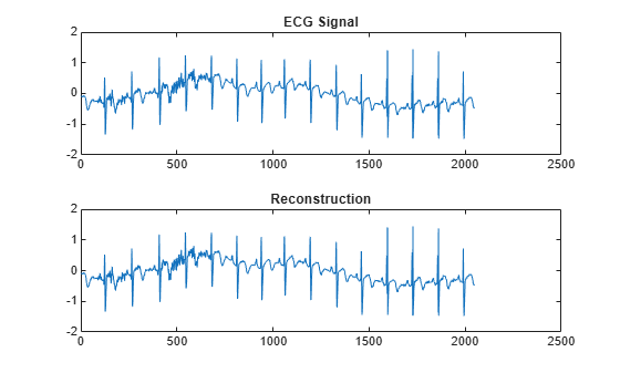
Obtain the MODWT of an ECG signal using the Fejér-Korovkin filters.
Load the ECG data.
load wecgCreate the 8-coefficient Fejér-Korovkin filters. Use the filters to obtain the MODWT of the ECG data.
[~,~,Lo,Hi] = wfilters("fk8");
wtecg = modwt(wecg,Lo,Hi);
Obtain the inverse MODWT using the filters.
xrec = imodwt(wtecg,Lo,Hi);
Obtain a second inverse MODWT using the wavelet name. Confirm both inverse transforms are equal.
xrec2 = imodwt(wtecg,"fk8");
max(abs(xrec-xrec2))
ans = 0
Plot the original data and one of the reconstructions.
subplot(2,1,1)
plot(wecg)
title("ECG Signal")
subplot(2,1,2)
plot(xrec)
title("Reconstruction")
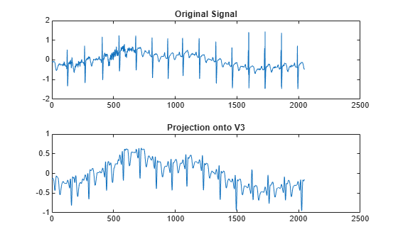
Obtain the MODWT of an ECG signal down to the maximum level and obtain the projection of the ECG signal onto the scaling space at level 3.
Load the ECG data.
load wecg;Obtain the MODWT.
wtecg = modwt(wecg);
Obtain the projection of the ECG signal onto , the scaling space at level three by using the imodwt function.
v3proj = imodwt(wtecg,3);
Plot the original signal and the projection.
subplot(2,1,1)
plot(wecg)
title('Original Signal')
subplot(2,1,2)
plot(v3proj)
title('Projection onto V3')
Note that the spikes characteristic of the R waves in the ECG are missing in the approximation. You can see the missing details by examining the wavelet coefficients at level three.
Plot the level-three wavelet coefficients.
figure
plot(wtecg(3,:))
title('Level-Three Wavelet Coefficients')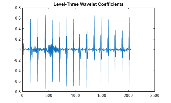
Obtain the inverse MODWT using reflection boundary handling for Southern Oscillation Index data. The sampling period is one day. imodwt with the 'reflection' option assumes that the input matrix, which is the modwt output, is twice the length of the original signal length. imodwt reflection boundary handling reduces the number of wavelet and scaling coefficients at each scale by half.
load soi;
wsoi = modwt(soi,4,'reflection');
xrecsoi = imodwt(wsoi,'reflection');
Use the L-infinity norm to show that the difference between the original signal and the reconstruction is extremely small. The largest absolute difference between the original signal and the reconstruction is on the order of , which demonstrates perfect reconstruction.
norm(abs(xrecsoi'-soi),Inf)
ans =
1.6433e-11
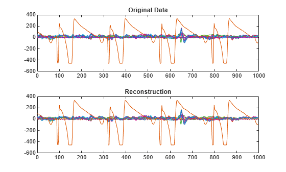
Load the 23 channel EEG data Espiga3 [2]. The channels are arranged column-wise. The data is sampled at 200 Hz.
load Espiga3Obtain the maximal overlap discrete wavelet transform down to the maximum level.
w = modwt(Espiga3);
Reconstruct the multichannel signal. Plot the original data and reconstruction.
xrec = imodwt(w);
subplot(2,1,1)
plot(Espiga3)
title('Original Data')
subplot(2,1,2)
plot(xrec)
title('Reconstruction')
Input Arguments
Output Arguments
References
[1] Percival, Donald B., and Andrew T. Walden. Wavelet Methods for Time Series Analysis. Cambridge Series in Statistical and Probabilistic Mathematics. Cambridge ; New York: Cambridge University Press, 2000.
[2] Mesa, Hector. “Adapted Wavelets for Pattern Detection.” In Progress in Pattern Recognition, Image Analysis and Applications, edited by Alberto Sanfeliu and Manuel Lazo Cortés, 3773:933–44. Berlin, Heidelberg: Springer Berlin Heidelberg, 2005. https://doi.org/10.1007/11578079_96.
Extended Capabilities
Version History
Introduced in R2015b