dualtree
Kingsbury Q-shift 1-D dual-tree complex wavelet transform
Description
[
returns the 1-D dual-tree complex wavelet transform (DTCWT) of A,D] = dualtree(X)X.
The output A is the matrix of
real-valued final-level scaling (lowpass) coefficients. The output D is
an L-by-1 cell array of complex-valued wavelet coefficients, where
L is the level of the transform.
The input X must have at least two samples. The DTCWT is obtained
by default down to level
floor(log2N), where
N is the length of X if X is
a vector and the row dimension of X if X is a
matrix. If N is odd, X is extended by one sample by
reflecting the last element of X.
By default, dualtree uses the near-symmetric biorthogonal filter
pair with lengths 5 (scaling filter) and 7 (wavelet filter) for level 1 and the orthogonal
Q-shift Hilbert wavelet filter pair of length 10 for levels greater than or equal to
2.
[___] = dualtree(
specifies additional options using name-value pair arguments. For example,
X,Name,Value)'Level',10 specifies a decomposition down to level 10.
Examples
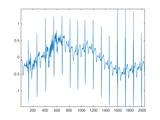
Load an ECG signal.
load wecg
plot(wecg)
axis tight
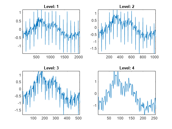
Obtain the 4-level dual-tree transform. Return the approximation (lowpass) coefficients at all levels.
[a,d,as] = dualtree(wecg,'Level',4);Plot the final-level wavelet coefficients from tree A and tree B.
figure
subplot(2,1,1)
plot(real(d{4}))
axis tight
title('Tree A')
subplot(2,1,2)
plot(imag(d{4}))
axis tight
title('Tree B')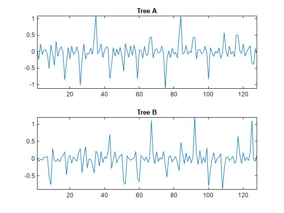
Plot the lowpass coefficients at each level of the transform.
figure
for k=1:4
    subplot(2,2,k)
    plot(as{k})
    axis tight
    title(['Level: ',num2str(k)])
end
This example shows that small signal shifts do not significantly change the distribution of energy among the DTCWT coefficients at different scales.
Load an ECG signal. The signal has 2048 samples.
load wecg
len = numel(wecg);
plot(wecg)
axis tight

Create two 1-by-3000 zero vectors. Insert the ECG signal into different segments of each zero vector.
shift1 = 328;
shift2 = 368;
vec1 = zeros(1,3000);
vec2 = zeros(1,3000);
vec1(shift1+[1:len]) = wecg;
vec2(shift2+[1:len]) = wecg;
Obtain the dual-tree transform of both vectors. Use default settings.
[a1,d1] = dualtree(vec1);
[a2,d2] = dualtree(vec2);
Compute the energy at each scale for both decompositions. Note that the energy distribution of the shifted signals across all scales remains approximately the same.
energy1 = cell2mat(cellfun(@(x)(sum(abs(x).^2)),d1,'uni',0));
energy2 = cell2mat(cellfun(@(x)(sum(abs(x).^2)),d2,'uni',0));
levels =cell(numel(energy1),1);
for k=1:numel(energy1)
    levels{k} = sprintf('Level %d',k);
end
energies = table(levels,energy1,energy2)
energies=11×3 table
       levels       energy1    energy2
    ____________    _______    _______

    {'Level 1' }    16.014     16.014
    {'Level 2' }    19.095     19.095
    {'Level 3' }     35.99      35.99
    {'Level 4' }    25.141     25.065
    {'Level 5' }     16.81     17.452
    {'Level 6' }    9.7078      9.161
    {'Level 7' }    2.3201     2.0513
    {'Level 8' }    8.3808     8.4197
    {'Level 9' }    23.006      22.56
    {'Level 10'}    70.764     73.964
    {'Level 11'}    64.097     59.022
Input Arguments
Name-Value Arguments
Output Arguments
References
[1] Antonini, M., M. Barlaud, P. Mathieu, and I. Daubechies. “Image Coding Using Wavelet Transform.” IEEE Transactions on Image Processing 1, no. 2 (April 1992): 205–20. https://doi.org/10.1109/83.136597.
[2] Kingsbury, Nick. “Complex Wavelets for Shift Invariant Analysis and Filtering of Signals.” Applied and Computational Harmonic Analysis 10, no. 3 (May 2001): 234–53. https://doi.org/10.1006/acha.2000.0343.
[3] Le Gall, D., and A. Tabatabai. “Sub-Band Coding of Digital Images Using Symmetric Short Kernel Filters and Arithmetic Coding Techniques.” In ICASSP-88., International Conference on Acoustics, Speech, and Signal Processing, 761–64. New York, NY, USA: IEEE, 1988. https://doi.org/10.1109/ICASSP.1988.196696.
Extended Capabilities
Version History
Introduced in R2020a