Unsupervised Anomaly Detection

This topic introduces the unsupervised anomaly detection features for multivariate sample data available in Statistics and Machine Learning Toolbox™, and describes the workflows of the features for outlier detection (detecting anomalies in training data) and novelty detection (detecting anomalies in new data with uncontaminated training data).

For unlabeled multivariate sample data, you can detect anomalies by using isolation forest, robust random cut forest, local outlier factor, one-class support vector machine (SVM), and Mahalanobis distance. These methods detect outliers either by training a model or by learning parameters. For novelty detection, you train a model or learn parameters with uncontaminated training data (data with no outliers) and detect anomalies in new data by using the trained model or learned parameters.

Isolation forest — The Isolation Forest algorithm detects anomalies by isolating them from normal points using an ensemble of isolation trees. Detect outliers by using the iforest function, and detect novelties by using the object function isanomaly.
Random robust cut forest — The Robust Random Cut Forest algorithm classifies a point as a normal point or an anomaly based on the changes in model complexity introduced by the point. Similar to the isolation forest algorithm, the robust random cut forest algorithm builds an ensemble of trees. The two algorithms differ in how they choose a split variable in trees and how they define anomaly scores. Detect outliers by using the rrcforest function, and detect novelties by using the object function isanomaly.
Local outlier factor — The Local Outlier Factor (LOF) algorithm detects anomalies based on the relative density of an observation with respect to the surrounding neighborhood. Detect outliers by using the lof function, and detect novelties by using the object function isanomaly.
One-class support vector machine (SVM) — One-class SVM, or unsupervised SVM, tries to separate data from the origin in the transformed high-dimensional predictor space. Detect outliers by using the ocsvm function, and detect novelties by using the object function isanomaly.
Mahalanobis Distance — If sample data follows a multivariate normal distribution, then the squared Mahalanobis distances from samples to the distribution follow a chi-square distribution. Therefore, you can use the distances to detect anomalies based on the critical values of the chi-square distribution. For outlier detection, use the robustcov function to compute robust Mahalanobis distances. For novelty detection, you can compute Mahalanobis distances by using the robustcov and pdist2 functions.

Outlier Detection

Open Live Script

This example illustrates the workflows of the five unsupervised anomaly detection methods (isolation forest, robust random cut forest, local outlier factor, one-class SVM, and Mahalanobis distance) for outlier detection.

Load Data

Load the humanactivity data set, which contains the variables feat and actid. The variable feat contains the predictor data matrix of 60 features for 24,075 observations, and the response variable actid contains the activity IDs for the observations as integers. This example uses the feat variable for anomaly detection.

load humanactivity

Find the size of the variable feat.

[N,D] = size(feat)

N = 24075

D = 60

Assume that the fraction of outliers in the data is 0.05.

contaminationFraction = 0.05;

Isolation Forest

Detect outliers by using the iforest function.

Train an isolation forest model by using the iforest function. Specify the fraction of outliers (ContaminationFraction) as 0.05.

rng("default") % For reproducibility
[forest,tf_forest,s_forest] = iforest(feat, ...
    ContaminationFraction=contaminationFraction);

forest is an IsolationForest object. iforest also returns the anomaly indicators (tf_forest) and anomaly scores (s_forest) for the data (feat). iforest determines the score threshold value (forest.ScoreThreshold) so that the function detects the specified fraction of observations as outliers.

Plot a histogram of the score values. Create a vertical line at the score threshold corresponding to the specified fraction.

figure
histogram(s_forest,Normalization="probability")
xline(forest.ScoreThreshold,"k-", ...
    join(["Threshold =" forest.ScoreThreshold]))
title("Histogram of Anomaly Scores for Isolation Forest")

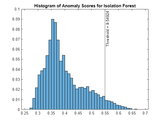
Figure contains an axes object. The axes object with title Histogram of Anomaly Scores for Isolation Forest contains 2 objects of type histogram, constantline.

Check the fraction of detected anomalies in the data.

OF_forest = sum(tf_forest)/N

OF_forest = 0.0496

The outlier fraction can be smaller than the specified fraction (0.05) when the scores have tied values at the threshold.

Robust Random Cut Forest

Detect outliers by using the rrcforest function.

Train a robust random cut forest model by using the rrcforest function. Specify the fraction of outliers (ContaminationFraction) as 0.05, and specify StandardizeData as true to standardize the input data.

rng("default") % For reproducibility
[rforest,tf_rforest,s_rforest] = rrcforest(feat, ...
    ContaminationFraction=contaminationFraction,StandardizeData=true);

rforest is a RobustRandomCutForest object. rrcforest also returns the anomaly indicators (tf_rforest) and anomaly scores (s_rforest) for the data (feat). rrcforest determines the score threshold value (rforest.ScoreThreshold) so that the function detects the specified fraction of observations as outliers.

Plot a histogram of the score values. Create a vertical line at the score threshold corresponding to the specified fraction.

figure
histogram(s_rforest,Normalization="probability")
xline(rforest.ScoreThreshold,"k-", ...
    join(["Threshold =" rforest.ScoreThreshold]))
title("Histogram of Anomaly Scores for Robust Random Cut Forest")

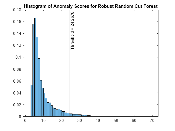
Figure contains an axes object. The axes object with title Histogram of Anomaly Scores for Robust Random Cut Forest contains 2 objects of type histogram, constantline.

Check the fraction of detected anomalies in the data.

OF_rforest = sum(tf_rforest)/N

OF_rforest = 0.0500

Local Outlier Factor

Detect outliers by using the lof function.

Train a local outlier factor model by using the lof function. Specify the fraction of outliers (ContaminationFraction) as 0.05, 500 nearest neighbors, and the Mahalanobis distance.

[LOFObj,tf_lof,s_lof] = lof(feat, ...
    ContaminationFraction=contaminationFraction, ...
    NumNeighbors=500,Distance="mahalanobis");

LOFObj is a LocalOutlierFactor object. lof also returns the anomaly indicators (tf_lof) and anomaly scores (s_lof) for the data (feat). lof determines the score threshold value (LOFObj.ScoreThreshold) so that the function detects the specified fraction of observations as outliers.

Plot a histogram of the score values. Create a vertical line at the score threshold corresponding to the specified fraction.

figure
histogram(s_lof,Normalization="probability")
xline(LOFObj.ScoreThreshold,"k-", ...
    join(["Threshold =" LOFObj.ScoreThreshold]))
title("Histogram of Anomaly Scores for Local Outlier Factor")

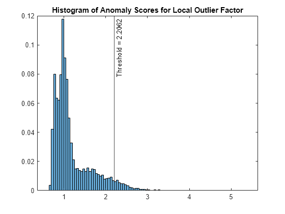
Figure contains an axes object. The axes object with title Histogram of Anomaly Scores for Local Outlier Factor contains 2 objects of type histogram, constantline.

Check the fraction of detected anomalies in the data.

OF_lof = sum(tf_lof)/N

OF_lof = 0.0500

One-Class SVM

Detect outliers by using the ocsvm function.

Train a one-class SVM model by using the ocsvm function. Specify the fraction of outliers (ContaminationFraction) as 0.05. In addition, set KernelScale to "auto" to let the function select an appropriate kernel scale parameter using a heuristic procedure, and specify StandardizeData as true to standardize the input data.

[Mdl,tf_OCSVM,s_OCSVM] = ocsvm(feat, ...
    ContaminationFraction=contaminationFraction, ...
    KernelScale="auto",StandardizeData=true);

Mdl is a OneClassSVM object. ocsvm also returns the anomaly indicators (tf_OCSVM) and anomaly scores (s_OCSVM) for the data (feat). ocsvm determines the score threshold value (Mdl.ScoreThreshold) so that the function detects the specified fraction of observations as outliers.

Plot a histogram of the score values. Create a vertical line at the score threshold corresponding to the specified fraction.

figure
histogram(s_OCSVM,Normalization="probability")
xline(Mdl.ScoreThreshold,"k-", ...
    join(["Threshold =" Mdl.ScoreThreshold]))
title("Histogram of Anomaly Scores for One-Class SVM")

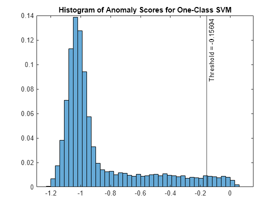
Figure contains an axes object. The axes object with title Histogram of Anomaly Scores for One-Class SVM contains 2 objects of type histogram, constantline.

Check the fraction of detected anomalies in the data.

OF_OCSVM = sum(tf_OCSVM)/N

OF_OCSVM = 0.0500

Mahalanobis Distance

Use the robustcov function to compute robust Mahalanobis distances and robust estimates for the mean and covariance of the data.

Compute the Mahalanobis distance from feat to the distribution of feat by using the robustcov function. Specify the fraction of outliers (OutlierFraction) as 0.05. robustcov minimizes the covariance determinant over 95% of the observations.

[sigma,mu,s_robustcov,tf_robustcov_default] = robustcov(feat, ...
    OutlierFraction=contaminationFraction);

robustcov finds the robust covariance matrix estimate (sigma) and robust mean estimate (mu), which are less sensitive to outliers than the estimates from the cov and mean functions. The robustcov function also computes the Mahalanobis distances (s_robustcov) and the outlier indicators (tf_robustcov_default). By default, the function assumes that the data set follows a multivariate normal distribution, and identifies 2.5% of input observations as outliers based on the critical values of the chi-square distribution.

If the data set satisfies the normality assumption, then the squared Mahalanobis distance follows a chi-square distribution with D degrees of freedom, where D is the dimension of the data. In that case, you can find a new threshold by using the chi2inv function to detect the specified fraction of observations as outliers.

s_robustcov_threshold = sqrt(chi2inv(1-contaminationFraction,D));
tf_robustcov = s_robustcov > s_robustcov_threshold;

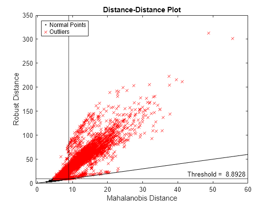
Create a distance-distance plot (DD plot) to check the multivariate normality of the data.

figure
d_classical = pdist2(feat,mean(feat),"mahalanobis");
gscatter(d_classical,s_robustcov,tf_robustcov,"kr",".x")
xline(s_robustcov_threshold,"k-")
yline(s_robustcov_threshold,"k-", ...
    join(["Threshold = " s_robustcov_threshold]));
l = refline([1 0]);
l.Color = "k";
xlabel("Mahalanobis Distance")
ylabel("Robust Distance")
legend("Normal Points","Outliers",Location="northwest")
title("Distance-Distance Plot")

Figure contains an axes object. The axes object with title Distance-Distance Plot, xlabel Mahalanobis Distance, ylabel Robust Distance contains 5 objects of type line, constantline. One or more of the lines displays its values using only markers These objects represent Normal Points, Outliers.

Zoom in the axes to see the normal points.

xlim([0 10])
ylim([0 10])

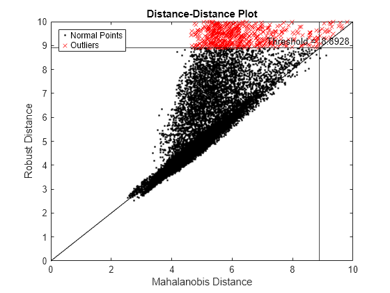
If a data set follows a multivariate normal distribution, then data points cluster tightly around the 45 degree reference line. The DD plot indicates that the data set does not follow a multivariate normal distribution.

Because the data set does not satisfy the normality assumption, use the quantile of the distance values for the cumulative probability (1 — contaminationFraction) to find a threshold.

s_robustcov_threshold = quantile(s_robustcov,1-contaminationFraction);

Obtain the anomaly indicators for feat using the new threshold s_robustcov_threshold.

tf_robustcov = s_robustcov > s_robustcov_threshold;

Check the fraction of detected anomalies in the data.

OF_robustcov = sum(tf_robustcov)/N

OF_robustcov = 0.0500

Compare Detected Outliers

To visualize the detected outliers, reduce the data dimension by using the tsne function.

rng("default") % For reproducibility
T = tsne(feat,Standardize=true,Perplexity=100,Exaggeration=20);

Plot the normal points and outliers in the reduced dimension. Compare the results of the five methods: the isolation forest algorithm, robust random cut forest algorithm, local outlier factor algorithm, one-class SVM model, and robust Mahalanobis distance from robustcov.

figure
tiledlayout(2,3)
nexttile
gscatter(T(:,1),T(:,2),tf_forest,"kr",[],[],"off")
title("Isolation Forest")
nexttile
gscatter(T(:,1),T(:,2),tf_rforest,"kr",[],[],"off")
title("Robust Random Cut Forest")
nexttile(4)
gscatter(T(:,1),T(:,2),tf_lof,"kr",[],[],"off")
title("Local Outlier Factor")
nexttile(5)
gscatter(T(:,1),T(:,2),tf_OCSVM,"kr",[],[],"off")
title("One-Class SVM")
nexttile(6)
gscatter(T(:,1),T(:,2),tf_robustcov,"kr",[],[],"off")
title("Robust Mahalanobis Distance")
l = legend("Normal Points","Outliers");
l.Layout.Tile = 3;

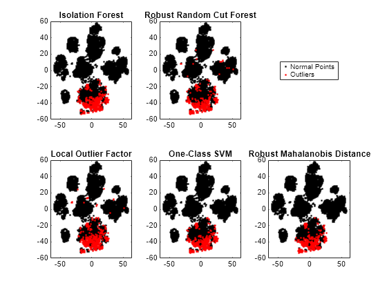
The novelties identified by the five methods are located near each other in the reduced dimension.

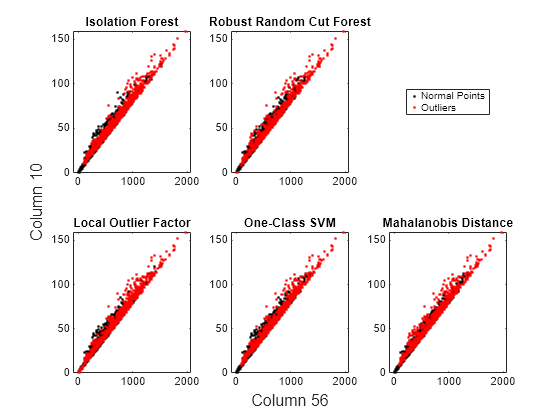
You can also visualize observation values using the two most important features selected by the fsulaplacian function.

idx = fsulaplacian(feat);
figure
t = tiledlayout(2,3);
nexttile
gscatter(feat(:,idx(1)),feat(:,idx(2)),tf_forest,"kr",[],[],"off")
title("Isolation Forest")
nexttile
gscatter(feat(:,idx(1)),feat(:,idx(2)),tf_rforest,"kr",[],[],"off")
title("Robust Random Cut Forest")
nexttile(4)
gscatter(feat(:,idx(1)),feat(:,idx(2)),tf_lof,"kr",[],[],"off")
title("Local Outlier Factor")
nexttile(5)
gscatter(feat(:,idx(1)),feat(:,idx(2)),tf_OCSVM,"kr",[],[],"off")
title("One-Class SVM")
nexttile(6)
gscatter(feat(:,idx(1)),feat(:,idx(2)),tf_robustcov,"kr",[],[],"off")
title("Mahalanobis Distance")
l = legend("Normal Points","Outliers");
l.Layout.Tile = 3;
xlabel(t,join(["Column" idx(1)]))
ylabel(t,join(["Column" idx(2)]))

Novelty Detection

Open Live Script

Load Data

load humanactivity

Partition the data into training and test sets by using the cvpartition function. Use 50% of the observations as training data and 50% of the observations as test data for novelty detection.

rng("default") % For reproducibility 
c = cvpartition(actid,Holdout=0.50);
trainingIndices = training(c); % Indices for the training set
testIndices = test(c); % Indices for the test set
XTrain = feat(trainingIndices,:);
XTest = feat(testIndices,:);

Assume that the training data is not contaminated (no outliers).

Find the size of the training and test sets.

[N,D] = size(XTrain)

N = 12038

D = 60

NTest = size(XTest,1)

NTest = 12037

Isolation Forest

Detect novelties using the object function isanomaly after training an isolation forest model by using the iforest function.

Train an isolation forest model.

[forest,tf_forest,s_forest] = iforest(XTrain);

forest is an IsolationForest object. iforest also returns the anomaly indicators (tf_forest) and anomaly scores (s_forest) for the training data (XTrain). By default, iforest treats all training observations as normal observations, and sets the score threshold (forest.ScoreThreshold) to the maximum score value.

Use the trained isolation forest model and the object function isanomaly to find novelties in XTest. The isanomaly function identifies observations with scores above the threshold (forest.ScoreThreshold) as novelties.

[tfTest_forest,sTest_forest] = isanomaly(forest,XTest);

The isanomaly function returns the anomaly indicators (tfTest_forest) and anomaly scores (sTest_forest) for the test data.

Plot histograms of the score values. Create a vertical line at the score threshold.

figure
histogram(s_forest,Normalization="probability")
hold on
histogram(sTest_forest,Normalization="probability")
xline(forest.ScoreThreshold,"k-", ...
    join(["Threshold =" forest.ScoreThreshold]))
legend("Training data","Test data",Location="southeast")
title("Histograms of Anomaly Scores for Isolation Forest")
hold off

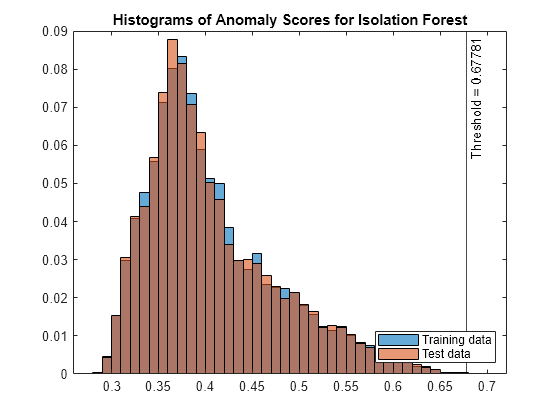
Figure contains an axes object. The axes object with title Histograms of Anomaly Scores for Isolation Forest contains 3 objects of type histogram, constantline. These objects represent Training data, Test data.

The anomaly score distribution of the test data is similar to that of the training data, so isanomaly detects a small number of anomalies in the test data.

Check the fraction of detected anomalies in the test data.

NF_forest = sum(tfTest_forest)/NTest

NF_forest = 8.3077e-05

Display the observation index of the anomalies in the test data.

idx_forest = find(tfTest_forest)

idx_forest = 3422

Robust Random Cut Forest

Detect novelties using the object function isanomaly after training a robust random cut forest model by using the rrcforest function.

Train a robust random cut forest model. Specify StandardizeData as true to standardize the input data.

[rforest,tf_rforest,s_rforest] = rrcforest(XTrain,StandardizeData=true);

rforest is a RobustRandomCutForest object. rrcforest also returns the anomaly indicators (tf_rforest) and anomaly scores (s_rforest) for the training data (XTrain). By default, rrcforest treats all training observations as normal observations, and sets the score threshold (rforest.ScoreThreshold) to the maximum score value.

Use the trained robust random cut forest model and the object function isanomaly to find novelties in XTest. The isanomaly function identifies observations with scores above the threshold (rforest.ScoreThreshold) as novelties.

[tfTest_rforest,sTest_rforest] = isanomaly(rforest,XTest);

The isanomaly function returns the anomaly indicators (tfTest_rforest) and anomaly scores (sTest_rforest) for the test data.

Plot histograms of the score values. Create a vertical line at the score threshold.

figure
histogram(s_rforest,Normalization="probability")
hold on
histogram(sTest_rforest,Normalization="probability")
xline(rforest.ScoreThreshold,"k-", ...
    join(["Threshold =" rforest.ScoreThreshold]))
legend("Training data","Test data",Location="southeast")
title("Histograms of Anomaly Scores for Robust Random Cut Forest")
hold off

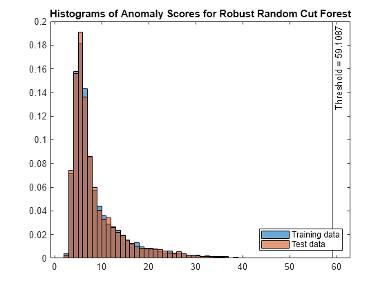
Figure contains an axes object. The axes object with title Histograms of Anomaly Scores for Robust Random Cut Forest contains 3 objects of type histogram, constantline. These objects represent Training data, Test data.

The anomaly score distribution of the test data is similar to that of the training data, so isanomaly detects a small number of anomalies in the test data.

Check the fraction of detected anomalies in the test data.

NF_rforest = sum(tfTest_rforest)/NTest

NF_rforest = 0

The anomaly score distribution of the test data is similar to that of the training data, so isanomaly does not detect any anomalies in the test data.

Local Outlier Factor

Detect novelties using the object function isanomaly after training a local outlier factor model by using the lof function.

Train a local outlier factor model.

[LOFObj,tf_lof,s_lof] = lof(XTrain);

LOFObj is a LocalOutlierFactor object. lof returns the anomaly indicators (tf_lof) and anomaly scores (s_lof) for the training data (XTrain). By default, lof treats all training observations as normal observations, and sets the score threshold (LOFObj.ScoreThreshold) to the maximum score value.

Use the trained local outlier factor model and the object function isanomaly to find novelties in XTest. The isanomaly function identifies observations with scores above the threshold (LOFObj.ScoreThreshold) as novelties.

[tfTest_lof,sTest_lof] = isanomaly(LOFObj,XTest);

The isanomaly function returns the anomaly indicators (tfTest_lof) and anomaly scores (sTest_lof) for the test data.

Plot histograms of the score values. Create a vertical line at the score threshold.

figure
histogram(s_lof,Normalization="probability")
hold on
histogram(sTest_lof,Normalization="probability")
xline(LOFObj.ScoreThreshold,"k-", ...
    join(["Threshold =" LOFObj.ScoreThreshold]))
legend("Training data","Test data",Location="southeast")
title("Histograms of Anomaly Scores for Local Outlier Factor")
hold off

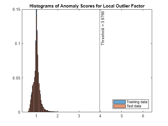
Figure contains an axes object. The axes object with title Histograms of Anomaly Scores for Local Outlier Factor contains 3 objects of type histogram, constantline. These objects represent Training data, Test data.

The anomaly score distribution of the test data is similar to that of the training data, so isanomaly detects a small number of anomalies in the test data.

Check the fraction of detected anomalies in the test data.

NF_lof = sum(tfTest_lof)/NTest

NF_lof = 8.3077e-05

Display the observation index of the anomalies in the test data.

idx_lof = find(tfTest_lof)

idx_lof = 8704

One-Class SVM

Detect novelties using the object function isanomaly after training a one-class SVM model by using the ocsvm function.

Train a one-class SVM model. Set KernelScale to "auto" to let the function select an appropriate kernel scale parameter using a heuristic procedure, and specify StandardizeData as true to standardize the input data.

[Mdl,tf_OCSVM,s_OCSVM] = ocsvm(XTrain, ...
    KernelScale="auto",StandardizeData=true);

Mdl is a OneClassSVM object. ocsvm returns the anomaly indicators (tf_OCSVM) and anomaly scores (s_OCSVM) for the training data (XTrain). By default, ocsvm treats all training observations as normal observations, and sets the score threshold (Mdl.ScoreThreshold) to the maximum score value.

Use the trained one-class SVM model and the object function isanomaly to find novelties in the test data (XTest). The isanomaly function identifies observations with scores above the threshold (Mdl.ScoreThreshold) as novelties.

[tfTest_OCSVM,sTest_OCSVM] = isanomaly(Mdl,XTest);

The isanomaly function returns the anomaly indicators (tfTest_OCSVM) and anomaly scores (sTest_OCSVM) for the test data.

Plot histograms of the score values. Create a vertical line at the score threshold.

figure
histogram(s_OCSVM,Normalization="probability")
hold on
histogram(sTest_OCSVM,Normalization="probability")
xline(Mdl.ScoreThreshold,"k-", ...
    join(["Threshold =" Mdl.ScoreThreshold]))
legend("Training data","Test data",Location="southeast")
title("Histograms of Anomaly Scores for One-Class SVM")
hold off

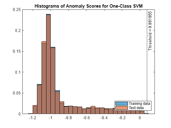
Figure contains an axes object. The axes object with title Histograms of Anomaly Scores for One-Class SVM contains 3 objects of type histogram, constantline. These objects represent Training data, Test data.

Check the fraction of detected anomalies in the test data.

NF_OCSVM = sum(tfTest_OCSVM)/NTest

NF_OCSVM = 1.6615e-04

Display the observation index of the anomalies in the test data.

idx_OCSVM = find(tfTest_OCSVM)

idx_OCSVM = 2×1

        3560
        8316

Mahalanobis Distance

Use the robustcov function to compute Mahalanobis distances of training data, and use the pdist2 function to compute Mahalanobis distances of test data.

Compute the Mahalanobis distance from XTrain to the distribution of XTrain by using the robustcov function. Specify the fraction of outliers (OutlierFraction) as 0.

[sigma,mu,s_mahal] = robustcov(XTrain,OutlierFraction=0);

robustcov also returns the estimates of covariance matrix (sigma) and mean (mu), which you can use to compute distances of test data.

Use the maximum value of s_mahal as the score threshold for novelty detection.

s_mahal_threshold = max(s_mahal);

Compute the Mahalanobis distance from XTest to the distribution of XTrain by using the pdist2 function.

sTest_mahal = pdist2(XTest,mu,"mahalanobis",sigma);

Obtain the anomaly indicators for XTest.

tfTest_mahal = sTest_mahal > s_mahal_threshold;

Plot histograms of the score values.

figure
histogram(s_mahal,Normalization="probability");
hold on
histogram(sTest_mahal,Normalization="probability");
xline(s_mahal_threshold,"k-", ...
    join(["Threshold =" s_mahal_threshold]))
legend("Training data","Test Data",Location="southeast")
title("Histograms of Mahalanobis Distances")
hold off

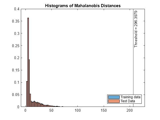
Figure contains an axes object. The axes object with title Histograms of Mahalanobis Distances contains 3 objects of type histogram, constantline. These objects represent Training data, Test Data.

Check the fraction of detected anomalies in the test data.

NF_mahal = sum(tfTest_mahal)/NTest

NF_mahal = 8.3077e-05

Display the observation index of the anomalies in the test data.

idx_mahal = find(tfTest_mahal)

idx_mahal = 3654