robustcov
Robust multivariate covariance and mean estimate
Syntax
Description
[___] = robustcov( returns
any of the arguments shown in the previous syntaxes, using additional
options specified by one or more x,Name,Value)Name,Value pair
arguments. For example, you can specify which robust estimator to
use or the start method to use for the attractors.
Examples
Use a Gaussian copula to generate random data points from a bivariate distribution.
rng default
rho = [1,0.05;0.05,1];
u = copularnd('Gaussian',rho,50);
Modify 5 randomly selected observations to be outliers.
noise = randperm(50,5);
u(noise,1) = u(noise,1)*5;
Calculate the robust covariance matrices using the three available methods: Fast-MCD, Orthogonalized Gnanadesikan-Kettenring (OGK), and Olive-Hawkins.
[Sfmcd, Mfmcd, dfmcd, Outfmcd] = robustcov(u);
[Sogk, Mogk, dogk, Outogk] = robustcov(u,'Method','ogk');
[Soh, Moh, doh, Outoh] = robustcov(u,'Method','olivehawkins');
Calculate the classical distance values for the sample data using the Mahalanobis measure.
d_classical = pdist2(u, mean(u),'mahal');
p = size(u,2);
chi2quantile = sqrt(chi2inv(0.975,p));
Create DD Plots for each robust covariance calculation method.
tiledlayout(2,2)
nexttile
plot(d_classical, dfmcd, 'o')
line([chi2quantile, chi2quantile], [0, 30], 'color', 'r')
line([0, 6], [chi2quantile, chi2quantile], 'color', 'r')
hold on
plot(d_classical(Outfmcd), dfmcd(Outfmcd), 'r+')
xlabel('Mahalanobis Distance')
ylabel('Robust Distance')
title('DD Plot, FMCD method')
hold off

nexttile
plot(d_classical, dogk, 'o')
line([chi2quantile, chi2quantile], [0, 30], 'color', 'r')
line([0, 6], [chi2quantile, chi2quantile], 'color', 'r')
hold on
plot(d_classical(Outogk), dogk(Outogk), 'r+')
xlabel('Mahalanobis Distance')
ylabel('Robust Distance')
title('DD Plot, OGK method')
hold off

nexttile
plot(d_classical, doh, 'o')
line([chi2quantile, chi2quantile], [0, 30], 'color', 'r')
line([0, 6], [chi2quantile, chi2quantile], 'color', 'r')
hold on
plot(d_classical(Outoh), doh(Outoh), 'r+')
xlabel('Mahalanobis Distance')
ylabel('Robust Distance')
title('DD Plot, Olive-Hawkins method')
hold off
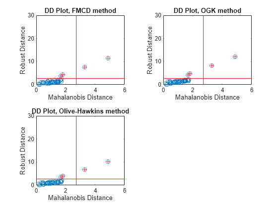
In a DD plot, the data points tend to cluster in a straight line that passes through the origin. Points that are far removed from this line are generally considered outliers. In each of the previous plots, the red '+' symbol indicates the data points that robustcov considers to be outliers.
This example shows how to use robustcov to evaluate sample data for multivariate normal or other elliptically-contoured (EC) distributions.
Generate random sample data from a multivariate normal distribution. Calculate the Mahalanobis distances for the robust covariance estimates (using the Olive-Hawkins method) and the classical covariance estimates.
rng('default')
x1 = mvnrnd(zeros(1,3),eye(3),200);
[~, ~, d1] = robustcov(x1,'Method','olivehawkins');
d_classical1 = pdist2(x1,mean(x1),'mahalanobis');
Generate random sample data from an elliptically-contoured (EC) distribution. Calculate the Mahalanobis distances for the robust covariance estimates (using the Olive-Hawkins method) and the classical covariance estimates.
mu1 = [0 0 0];
sig1 = eye(3);
mu2 = [0 0 0];
sig2 = 25*eye(3);
x2 = [mvnrnd(mu1,sig1,120);mvnrnd(mu2,sig2,80)];
[~, ~, d2] = robustcov(x2, 'Method','olivehawkins');
d_classical2 = pdist2(x2, mean(x2), 'mahalanobis');
Generate random sample data from a multivariate lognormal distribution, which is neither multivariate normal or elliptically-contoured. Calculate the Mahalanobis distances for the robust covariance estimates (using the Olive-Hawkins method) and the classical covariance estimates.
x3 = exp(x1);
[~, ~, d3] = robustcov(x3, 'Method','olivehawkins');
d_classical3 = pdist2(x3, mean(x3), 'mahalanobis');
Create a D-D Plot for each of the three sets of sample data to compare.
figure
subplot(2,2,1)
plot(d_classical1,d1, 'o')
line([0 4.5], [0, 4.5])
xlabel('Mahalanobis Distance')
ylabel('Robust Distance')
title('DD Plot, Multivariate Normal')

subplot(2,2,2)
plot(d_classical2, d2, 'o')
line([0 18], [0, 18])
xlabel('Mahalanobis Distance')
ylabel('Robust Distance')
title('DD Plot, Elliptically-Contoured')

subplot(2,2,3)
plot(d_classical3, d3, 'o')
line([0 18], [0, 18])
xlabel('Mahalanobis Distance')
ylabel('Robust Distance')
title('DD Plot, 200 Lognormal cases')
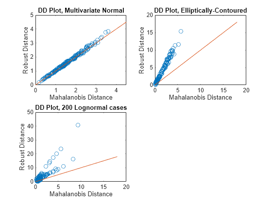
For data with a multivariate normal distribution (as shown in the upper left), the plotted points follow a straight, 45-degree line extending from the origin. For data with an elliptically-contoured distribution (as shown in the upper right), the plotted points follow a straight line, but are not at a 45-degree angle to the origin. For the lognormal distribution (as shown in the lower left), the plotted points do not follow a straight line.
It is difficult to identify any pattern in the lognormal distribution plot because most of the points are in the lower left of the plot. Use a weighted DD plot to magnify this corner and reveal features that are obscured when large robust distances exist.
d3_weighted = d3(d3 < sqrt(chi2inv(0.975,3)));
d_classical_weighted = d_classical3(d3 < sqrt(chi2inv(0.975,3)));
Add a fourth subplot to the figure to show the results of the weighting process on the lognormally distributed data.
subplot(2,2,4)
plot(d_classical_weighted, d3_weighted, 'o')
line([0 3], [0, 3])
xlabel('Mahalanobis Distance')
ylabel('Robust Distance')
title('Weighted DD Plot, 200 Lognormal cases')
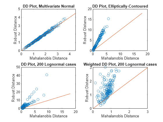
The scale on this plot indicates that it represents a magnified view of the original DD plot for the lognormal data. This view more clearly shows the lack of pattern to the plot, which indicates that the data is neither multivariate normal nor elliptically contoured.
Use a Gaussian copula to generate random data points from a bivariate distribution.
rng default
rho = [1,0.05;0.05,1];
u = copularnd('Gaussian',rho,50);
Modify 5 randomly selected observations to be outliers.
noise = randperm(50,5);
u(noise,1) = u(noise,1)*5;
Visualize the bivariate data using a scatter plot.
figure
scatter(u(:,1),u(:,2))
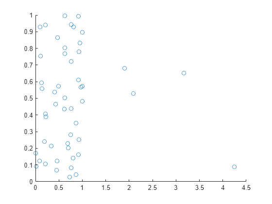
Most of the data points appear on the left side of the plot. However, some of the data points appear further to the right. These points are possible outliers that could affect the covariance matrix calculation.
Compare the classical and robust covariance matrices.
c = cov(u)
c = 2×2

    0.5523    0.0000
    0.0000    0.0913
rc = robustcov(u)
rc = 2×2

    0.1117    0.0364
    0.0364    0.1695
The classical and robust covariance matrices differ because the outliers present in the sample data influence the results.
Identify and plot the data points that robustcov considers outliers.
[sig,mu,mah,outliers] = robustcov(u);
figure
gscatter(u(:,1),u(:,2),outliers,'br','ox')
legend({'Not outliers','Outliers'})
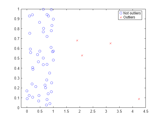
robustcov identifies the data points on the right side of the plot as potential outliers, and treats them accordingly when calculating the robust covariance matrix.
Input Arguments
Sample data used to estimate the robust covariance matrix, specified
as a matrix of numeric values. x is an n-by-p matrix
where each row is an observation and each column is a variable.
robustcov removes any rows with missing
predictor values when calculating the robust covariance matrix.
Data Types: single | double
Name-Value Arguments
Specify optional pairs of arguments as
Name1=Value1,...,NameN=ValueN, where Name is
the argument name and Value is the corresponding value.
Name-value arguments must appear after other arguments, but the order of the
pairs does not matter.
Before R2021a, use commas to separate each name and value, and enclose
Name in quotes.
Example: 'Method','ogk','NumOGKIterations',1 specifies the robust estimator
as the Orthogonalized Gnanadesikan-Kettenring method and sets the number of
orthogonalization iterations to 1.
For All Estimators
Robust estimator, specified as one of the following.
| Name | Value |
|---|---|
'fmcd' | FAST-MCD (Minimum Covariance Determinant) method |
'ogk' | Orthogonalized Gnanadesikan-Kettenring (OGK) estimate |
'olivehawkins' | Concentration algorithm techniques, a family of fast, consistent and highly outlier-resistant methods |
Example: 'Method','ogk'
For the FMCD and OliveHawkins Methods Only
Outlier fraction, specified as the comma-separated pair consisting
of 'OutlierFraction' and a numeric value in the
range [0,0.5]. The value 1 – OutlierFraction specifies
the fraction of observations over which to minimize the covariance
determinant.
The algorithm chooses a subsample of size h =
ceiling(n + p + 1) / 2),
where n is the number of observations and p is
the number of dimensions. OutlierFraction is the
value for which the maximum possible breakdown is achieved, and controls
the size of the subsets h over which the covariance
determinant is minimized. The algorithm then chooses h to
approximately equal (1 – OutlierFraction)
× n observations per
subset.
Example: 'OutlierFraction',0.25
Data Types: single | double
Number of trials, specified as the comma-separated pair consisting
of 'NumTrials' and a positive integer value.
If 'Method' is 'fmcd',
then NumTrials is the number of random subsamples
of size (p + 1)
drawn from the sample data as starting points in the algorithm. p is
the number of dimensions in the sample data. In this case, the default
value for NumTrials is 500.
If 'Method' is 'olivehawkins',
then NumTrials is the number of trial fits, or
attractors, to be used. In this case, the default value for NumTrials is
2. This option is only useful for non-deterministic starts.
Example: 'NumTrials',300
Data Types: single | double
For the FMCD Method Only
Flag to apply small-sample correction factor, specified as the
comma-separated pair consisting of 'BiasCorrection' and
either 1 or 0. A 1 value
indicates that robustcov corrects for bias in
the covariance estimate for small samples. A 0 value
indicates that robustcov does not apply this
correction.
Example: 'BiasCorrection',0
Data Types: logical
For the OGK Method Only
Number of orthogonalization iterations, specified as the comma-separated
pair consisting of 'NumOGKIterations' and a positive
integer value. Generally, this value is set to 1 or 2, and further
steps are unlikely to improve the estimation.
Example: 'NumIter',1
Data Types: single | double
Function for computing univariate robust estimates, specified
as the comma-separated pair consisting of 'UnivariateEstimator' and
one of the following.
| Name | Value |
|---|---|
'tauscale' | Use the “tau-scale” estimate of Yohai and Zamar, which is a truncated standard deviation and a weighted mean. |
'qn' | Use the Qn scale estimate of Croux and Rousseeuw. |
Example: 'UnivariateEstimator','qn'
For the OliveHawkins Method Only
Method for reweighting in the efficiency step, specified as
the comma-separated pair consisting of 'ReweightingMethod' and
one of the following.
| Name | Value |
|---|---|
'rfch' | Uses two reweighting steps. This is a standard method of reweighting to improve efficiency. |
'rmvn' | Reweighted multivariate normal. Uses two reweighting steps that can be useful for estimating the true covariance matrix under a variety of outlier configurations when the clean data are multivariate normal. |
Example: 'ReweightingMethod','rmvn'
Number of concentration steps, specified as the comma-separated
pair consisting of 'NumConcentrationSteps' and
a positive integer value.
Example: 'NumConcentrationSteps',8
Data Types: single | double
Start method for each attractor, specified as the comma-separated
pair consisting of 'Start' and one of the following.
| Name | Value |
|---|---|
'classical' | Use the classical estimator as the start. This is the DGK attractor which, used on its own, is known as the DGK estimator. |
'medianball' | Use the Median Ball as the start. The Median Ball is (med(x),eye(p)).
So 50% of cases furthest in Euclidean distance from the sample median
are trimmed for computing the MB start. This is the MB attractor which,
used on its own, is known as the MB estimator. |
'elemental' | The attractor is generated by concentration where the start is a randomly selected elemental start: the classical estimator applied to a randomly selected “elemental set” of p + 1 cases. This “elemental” attractor is computationally efficient, but suffers from theoretical drawbacks, as it is inconsistent and zero breakdown. |
By default, the attractor is chosen as follows: If one of the
attractors is 'medianball', then any attractor
whose location estimate has greater Euclidean distance from median(X) than
half the data (in other words, is outside the median ball) is not
used. Then the final attractor is chosen based on the MCD criterion.
You can also specify a function handle for a function that returns two output arguments used for computing the initial location and scatter estimates..
You can also specify a cell array containing any combination of the options given in the previous table and function handles. The number of attractors used is equal to the length of the cell array. This option allows more control over the algorithm and the ability to specify a custom number of attractors and starts.
Example: 'StartMethod','medianball'
Output Arguments
Robust covariance matrix estimates, returned as a p-by-p numeric matrix. p is the number of predictors contained in the sample data.
Robust mean estimates, returned as a 1-by-p array of numeric values. p is the number of predictors contained in the sample data.
Robust Mahalanobis distances, returned as a 1-by-n
array of numeric values. robustcov removes any rows of
x that contain missing data, so the number of rows
of mah might be smaller than the number of rows in
x.
Indices of observations retained as outliers in the sample data x,
returned as a 1-by-n array of logical values. A 0 value
indicates that the observation is not an outlier. A 1 value
indicates that the observation is an outlier.
robustcov removes any rows of x that
contain missing data, so the number of rows of outliers might
be smaller than the number of rows in x.
Structure containing estimate information, returned as a structure.
More About
The Mahalanobis distance is a measure between a sample point and a distribution.
The Mahalanobis distance from a vector x to a distribution with mean μ and covariance Σ is
The distance represents how far x is from the mean in number of standard deviations.
robustcov returns the robust Mahalanobis distances
(mah) from observations in x to the
distribution with mean mu and covariance
sig.
Algorithms
Minimum covariance determinant (MCD) is
the fastest estimator of multivariate location and scatter that is
both consistent and robust. However, an exact evaluation of the MCD
is impractical because it is computationally expensive to evaluate
all possible subsets of the sample data. robustcov uses
the FAST-MCD method to implement MCD [3]
The FAST-MCD method selects h observations out of n (where n/2 < h ≤ n) whose classical covariance matrix has the lowest possible determinant. The MCD mean is the mean of the h selected observations.
The MCD covariance is the covariance matrix of the h selected points, multiplied by a consistency factor to obtain consistency at the multivariate normal distribution, and by a correction factor to correct for bias at small sample sizes.
Orthogonalized Gnanadesikan-Kettenring (OGK) estimate is a positive definite estimate of the scatter starting from the Gnanadesikan and Kettering (GK) estimator, a pairwise robust scatter matrix that may be non-positive definite [1]. The estimate uses a form of principal components called an orthogonalization iteration on the pairwise scatter matrix, replacing its eigenvalues, which could be negative, with robust variances. This procedure can be iterated for improved results, and convergence is usually obtained after 2 or 3 iterations.
The Olive-Hawkins estimate uses the “concentration algorithm” techniques proposed by Olive and Hawkins. This is a family of fast, consistent, and highly outlier-resistant methods. The estimate is a robust root n-consistent estimator of covariance for elliptically contoured distributions with fourth moments. This estimate is obtained by first generating trial estimates, or starts, and then using the concentration technique from each trial fit to obtain attractors.
Suppose (T0j,C0j) is a start, then at the next iteration the classical mean and covariance estimators are computed from the approximately n / 2 cases (where n is the number of observations) with the smallest Mahalanobis distances based on the estimates from the previous iteration. This iteration can be continued for a fixed number of steps k, with the estimate at the last step, k, being the attractor. The final estimate is chosen based on a given criterion.
By default, two attractors are used. The first attractor is
the Devlin-Gnanadesikan-Kettering (DGK) attractor, where the start
used is the classical estimator. The second attractor is the Median
Ball (MB) attractor, where the start used is (median(x),eye(p)),
in other words the half set of data closest to median(x) in
Euclidean distance. The MB attractor is used if the location estimator
of the DGK attractor is outside of the median ball, and the attractor
with the smallest determinant is used otherwise. The final mean estimate
is the mean estimate of the chosen attractor, and the final covariance
estimate is the covariance estimate of the chosen attractor, multiplied
by a scaling factor to make the estimate consistent at the normal
distribution.
References
[1] Maronna, R. and Zamar, R.H.. “Robust estimates of location and dispersion for high-dimensional datasets.” Technometrics, Vol. 50, 2002.
[2] Pison, S. Van Aelst and G. Willems. “Small Sample Corrections for LTS and MCD.” Metrika, Vol. 55, 2002.
[3] Rousseeuw, P.J. and Van Driessen, K. “A fast algorithm for the minimum covariance determinant estimator.” Technometrics, Vol. 41, 1999.
[4] Olive, D.J. “A resistant estimator of multivariate location and dispersion.” Computational Statistics and Data Analysis, Vol. 46, pp. 99–102, 2004.
Extended Capabilities
The robustcov function fully supports
thread-based environments. For more information, see Run MATLAB Functions in Thread-Based Environment.
Version History
Introduced in R2016a
MATLAB Command
You clicked a link that corresponds to this MATLAB command:
Run the command by entering it in the MATLAB Command Window. Web browsers do not support MATLAB commands.
Select a Web Site
Choose a web site to get translated content where available and see local events and offers. Based on your location, we recommend that you select: .
You can also select a web site from the following list
How to Get Best Site Performance
Select the China site (in Chinese or English) for best site performance. Other MathWorks country sites are not optimized for visits from your location.
Americas
- América Latina (Español)
- Canada (English)
- United States (English)
Europe
- Belgium (English)
- Denmark (English)
- Deutschland (Deutsch)
- España (Español)
- Finland (English)
- France (Français)
- Ireland (English)
- Italia (Italiano)
- Luxembourg (English)
- Netherlands (English)
- Norway (English)
- Österreich (Deutsch)
- Portugal (English)
- Sweden (English)
- Switzerland
- United Kingdom (English)