Anomaly Detection with Isolation Forest
Introduction to Isolation Forest
The isolation forest algorithm [1] detects anomalies by isolating anomalies from normal points using an ensemble of isolation trees. Each isolation tree is trained for a subset of training observations, sampled without replacements. The algorithm grows an isolation tree by choosing a split variable and split position at random until every observation in a subset lands in a separate leaf node. Anomalies are few and different; therefore, an anomaly lands in a separate leaf node closer to the root node and has a shorter path length (the distance from the root node to the leaf node) than normal points. The algorithm identifies anomalies using anomaly scores defined based on the average path lengths over all isolation trees.
Use the iforest
function, IsolationForest object, and isanomaly object function for outlier detection and novelty
detection.
Outlier detection (detecting anomalies in training data) — Detect anomalies in training data by using the
iforestfunction.iforestbuilds anIsolationForestobject and returns anomaly indicators and scores for the training data. For an example, see Detect Outliers.Novelty detection (detecting anomalies in new data with uncontaminated training data) — Create an
IsolationForestobject by passing uncontaminated training data (data with no outliers) toiforest, and detect anomalies in new data by passing the object and the new data to the object functionisanomaly. For each observation of the new data, the function finds the average path length to reach a leaf node from the root node in the trained isolation forest, and returns an anomaly indicator and score. For an example, see Detect Novelties.
Parameters for Isolation Forests
You can specify parameters for the isolation forest algorithm by using the
name-value arguments of iforest:
NumObservationsPerLearner(number of observations for each isolation tree) — Each isolation tree corresponds to a subset of training observations. For each tree,iforestsamplesmin(N,256)number of observations from the training data without replacement, whereNis the number of training observations. The isolation forest algorithm performs well with a small sample size because it helps to detect dense anomalies and anomalies close to normal points. However, you need to experiment with the sample size ifNis small. For an example, see Examine NumObservationsPerLearner for Small Data.NumLearners(number of isolation trees) — By default, theiforestfunction grows 100 isolation trees for the isolation forest because the average path lengths usually converge well before growing 100 isolation trees [1].
Anomaly Scores
The isolation forest algorithm computes the anomaly score s(x) of an observation x by normalizing the path length h(x):
where E[h(x)] is the average path length over all isolation trees in the isolation forest, and c(n) is the average path length of unsuccessful searches in a binary search tree of n observations.
The score approaches 1 as E[h(x)] approaches 0. Therefore, a score value close to 1 indicates an anomaly.
The score approaches 0 as E[h(x)] approaches n – 1. Also, the score approaches 0.5 when E[h(x)] approaches c(n). Therefore, a score value smaller than 0.5 and close to 0 indicates a normal point.
Anomaly Indicators
iforest and isanomaly identify
observations with anomaly scores above the score threshold as anomalies. The
functions return a logical vector that has the same length as the input data. A
value of logical 1 (true) indicates that the corresponding row of
the input data is an anomaly.
iforestdetermines the threshold value (ScoreThresholdproperty value) to detect the specified fraction (ContaminationFractionname-value argument) of training observations as anomalies. By default, the function treats all training observations as normal observations.isanomalyprovides theScoreThresholdname-value argument, which you can use to specify the threshold. The default threshold is the value determined when the isolation forest is trained.
Detect Outliers and Plot Contours of Anomaly Scores
This example uses generated sample data containing outliers. Train an isolation forest model and detect the outliers by using the iforest function. Then, compute anomaly scores for the points around the sample data by using the isanomaly function, and create a contour plot of the anomaly scores.
Generate Sample Data
Use a Gaussian copula to generate random data points from a bivariate distribution.
rng("default")
rho = [1,0.05;0.05,1];
n = 1000;
u = copularnd("Gaussian",rho,n);
Add noise to 5% of randomly selected observations to make the observations outliers.
noise = randperm(n,0.05*n);
true_tf = false(n,1);
true_tf(noise) = true;
u(true_tf,1) = u(true_tf,1)*5;
Train Isolation Forest and Detect Outliers
Train an isolation forest model by using the iforest function. Specify the fraction of anomalies in the training observations as 0.05.
[f,tf,scores] = iforest(u,ContaminationFraction=0.05);
f is an IsolationForest object. iforest also returns the anomaly indicators (tf) and anomaly scores (scores) for the training data.
Plot a histogram of the score values. Create a vertical line at the score threshold corresponding to the specified fraction.
histogram(scores)
xline(f.ScoreThreshold,"r-",join(["Threshold" f.ScoreThreshold]))

Plot Contours of Anomaly Scores
Use the trained isolation forest model and the isanomaly function to compute anomaly scores for 2-D grid coordinates around the training observations.
l1 = linspace(min(u(:,1),[],1),max(u(:,1),[],1));
l2 = linspace(min(u(:,2),[],1),max(u(:,2),[],1));
[X1,X2] = meshgrid(l1,l2);
[~,scores_grid] = isanomaly(f,[X1(:),X2(:)]);
scores_grid = reshape(scores_grid,size(X1,1),size(X2,2));
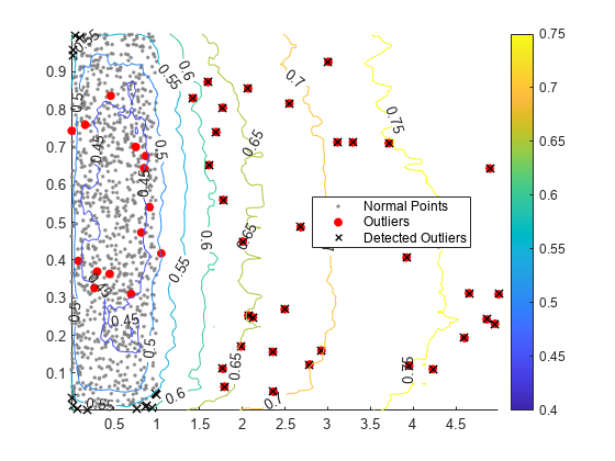
Create a scatter plot of the training observations and a contour plot of the anomaly scores. Flag true outliers and the outliers detected by iforest.
idx = setdiff(1:1000,noise);
scatter(u(idx,1),u(idx,2),[],[0.5 0.5 0.5],".")
hold on
scatter(u(noise,1),u(noise,2),"ro","filled")
scatter(u(tf,1),u(tf,2),60,"kx",LineWidth=1)
contour(X1,X2,scores_grid,"ShowText","on")
legend(["Normal Points" "Outliers" "Detected Outliers"],Location="best")
colorbar
hold off
Check Performance
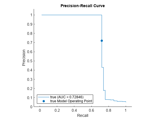
Check the performance of iforest by plotting a precision-recall curve and computing the area under the curve (AUC) value. Create a rocmetrics object. rocmetrics computes the false positive rates and the true positive rates (or recall) by default. Specify the AdditionalMetrics name-value argument to additionally compute the precision values (or positive predictive values).
rocObj = rocmetrics(true_tf,scores,true,AdditionalMetrics="PositivePredictiveValue");Plot the curve by using the plot function of rocmetrics. Specify the y-axis metric as precision (or positive predictive value) and the x-axis metric as recall (or true positive rate). Display a filled circle at the model operating point corresponding to f.ScoreThreshold. Compute the area under the precision-recall curve using the trapezoidal method of the trapz function, and display the value in the legend.
r = plot(rocObj,YAxisMetric="PositivePredictiveValue",XAxisMetric="TruePositiveRate");
hold on
idx = find(rocObj.Metrics.Threshold>=f.ScoreThreshold,1,'last');
scatter(rocObj.Metrics.TruePositiveRate(idx), ...
    rocObj.Metrics.PositivePredictiveValue(idx), ...
    [],r.Color,"filled")
xyData = rmmissing([r.XData r.YData]);
auc = trapz(xyData(:,1),xyData(:,2));
legend(join([r.DisplayName " (AUC = " string(auc) ")"],""),"true Model Operating Point")
xlabel("Recall")
ylabel("Precision")
title("Precision-Recall Curve")
hold off
Examine NumObservationsPerLearner for Small Data
For each isolation tree, iforest samples min(N,256) number of observations from the training data without replacement, where N is the number of training observations. Keeping the sample size small helps to detect dense anomalies and anomalies close to normal points. However, you need to experiment with the sample size if N is small.
This example shows how to train isolation forest models for small data with various sample sizes, create plots of anomaly score values versus sample sizes, and visualize identified anomalies.
Load Sample Data
Load Fisher's iris data set.
load fisheririsThe data contains four measurements (sepal length, sepal width, petal length, and petal width) from three species of iris flowers. The matrix meas contains all four measurements for 150 flowers.
Train Isolation Forest with Various Sample Sizes
Train isolation forest models with various sample sizes, and obtain anomaly scores for the training observations.
s = NaN(150,150);
rng("default")
for i = 3: 150
    [~,~,s(:,i)] = iforest(meas,NumObservationsPerLearner=i);
end
Divide the observations into three groups based on the average scores, and create plots of anomaly scores versus sample sizes.
score_threshold1 = 0.5;
score_threshold2 = 0.55;

m = mean(s,2,"omitnan");
ind1 = find(m < score_threshold1);
ind2 = find(m <= score_threshold2 & m >= score_threshold1);
ind3 = find(m > score_threshold2);

figure
t = tiledlayout(3,1);
nexttile
plot(s(ind1,:)')
title(join(["Observations with average score <  " score_threshold1]))
nexttile
plot(s(ind2,:)')
title(join(["Observations with average score in [" ...
    score_threshold1 " " score_threshold2 "]"]))
nexttile
plot(s(ind3,:)')
title(join(["Observations with average score >  " score_threshold2]))
xlabel(t,"Number of Observations for Each Tree")
ylabel(t,"Anomaly Score")
![Figure contains 3 axes objects. Axes object 1 with title Observations with average score < 0.5 contains 101 objects of type line. Axes object 2 with title Observations with average score in [ 0.5 0.55 ] contains 33 objects of type line. Axes object 3 with title Observations with average score > 0.55 contains 16 objects of type line.](../examples/stats/win64/ExamineNumObservationsPerLearnerForSmallDataExample_01.png)
The anomaly score decreases as the sample size increases for the observations whose average score values are less than 0.5. For the observations whose average score values are greater than 0.55, the anomaly score increases as the sample size increases and then the score converges roughly when the sample size reaches 50.
Detect anomalies in training observations by using isolation forest models with the sample sizes 50 and 100. Specify the fraction of anomalies in the training observations as 0.05.
[f1,tf1,scores1] = iforest(meas,NumObservationsPerLearner=50, ...
    ContaminationFraction=0.05);
[f2,tf2,scores2] = iforest(meas,NumObservationsPerLearner=100, ...
    ContaminationFraction=0.05);
Display the observation indexes of the anomalies.
find(tf1)
ans = 7×1

    14
    42
   110
   118
   119
   123
   132
find(tf2)
ans = 7×1

    14
    15
    16
   110
   118
   119
   132
The two isolation forest models have five anomalies in common.
Visualize Anomalies
For the isolation forest model with the sample size 50, visually compare observation values between normal points and anomalies. Create a matrix of grouped histograms and grouped scatter plots for each combination of variables by using the gplotmatrix function.
tf1 = categorical(tf1,[0 1],["Normal Points" "Anomalies"]);
predictorNames = ["Sepal Length" "Sepal Width" ...
    "Petal Length" "Petal Width"];
gplotmatrix(meas,[],tf1,"kr",".x",[],[],[],predictorNames)

For high-dimensional data, you can visualize data by using only the important features. You can also visualize data after reducing the dimension by using t-SNE (t-Distributed Stochastic Neighbor Embedding).
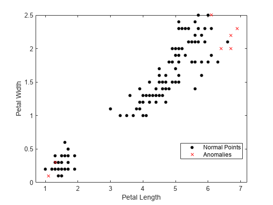
Visualize observation values using the two most important features selected by the fsulaplacian function.
idx = fsulaplacian(meas)
idx = 1×4

     3     4     1     2
gscatter(meas(:,idx(1)),meas(:,idx(2)),tf1,"kr",".x",[],"on", ...
    predictorNames(idx(1)),predictorNames(idx(2)))
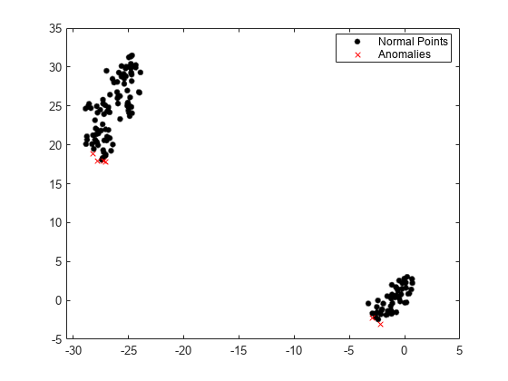
Visualize observation values after reducing the dimension by using the tsne function.
Y = tsne(meas);
gscatter(Y(:,1),Y(:,2),tf1,"kr",".x")
References
[1] Liu, F. T., K. M. Ting, and Z. Zhou. "Isolation Forest," 2008 Eighth IEEE International Conference on Data Mining. Pisa, Italy, 2008, pp. 413-422.
See Also
iforest | IsolationForest | isanomaly