Reduce Outlier Effects Using Robust Regression
You can reduce outlier effects in linear regression models by using robust linear regression. This topic defines robust regression, shows how to use it to fit a linear model, and compares the results to a standard fit. You can use fitlm with the 'RobustOpts' name-value pair argument to fit a robust regression model. Or you can use robustfit to simply compute the robust regression coefficient parameters.
Why Use Robust Regression?
Robust linear regression is less sensitive to outliers than standard linear regression. Standard linear regression uses ordinary least-squares fitting to compute the model parameters that relate the response data to the predictor data with one or more coefficients. (See Estimation of Multivariate Regression Models for more details.) As a result, outliers have a large influence on the fit, because squaring the residuals magnifies the effects of these extreme data points. Models that use standard linear regression, described in What Is a Linear Regression Model?, are based on certain assumptions, such as a normal distribution of errors in the observed responses. If the distribution of errors is asymmetric or prone to outliers, model assumptions are invalidated, and parameter estimates, confidence intervals, and other computed statistics become unreliable.
Robust regression uses a method called iteratively reweighted least squares to assign a weight to each data point. This method is less sensitive to large changes in small parts of the data. As a result, robust linear regression is less sensitive to outliers than standard linear regression.
Iteratively Reweighted Least Squares
In weighted least squares, the fitting process includes the weight as an additional scale factor, which improves the fit. The weights determine how much each response value influences the final parameter estimates. A low-quality data point (for example, an outlier) should have less influence on the fit. To compute the weights wi, you can use predefined weight functions, such as Tukey's bisquare function (see the name-value pair argument 'RobustOpts' in fitlm for more options).
The iteratively reweighted least-squares algorithm automatically and iteratively calculates the weights. At initialization, the algorithm assigns equal weight to each data point, and estimates the model coefficients using ordinary least squares. At each iteration, the algorithm computes the weights wi, giving lower weight to points farther from model predictions in the previous iteration. The algorithm then computes model coefficients b using weighted least squares. Iteration stops when the values of the coefficient estimates converge within a specified tolerance. This algorithm simultaneously seeks to find the curve that fits the bulk of the data using the least-squares approach, and to minimize the effects of outliers.
For more details, see Steps for Iteratively Reweighted Least Squares.
Compare Results of Standard and Robust Least-Squares Fit
This example shows how to use robust regression with the fitlm function, and compares the results of a robust fit to a standard least-squares fit.
Load the moore data. The predictor data is in the first five columns, and the response data is in the sixth.
load moore
X = moore(:,1:5);
y = moore(:,6);
Fit the least-squares linear model to the data.
mdl = fitlm(X,y)
mdl =
Linear regression model:
    y ~ 1 + x1 + x2 + x3 + x4 + x5

Estimated Coefficients:
                    Estimate          SE          tStat       pValue
                   ___________    __________    _________    ________

    (Intercept)        -2.1561       0.91349      -2.3603      0.0333
    x1             -9.0116e-06    0.00051835    -0.017385     0.98637
    x2               0.0013159     0.0012635       1.0415     0.31531
    x3               0.0001278    7.6902e-05       1.6618     0.11876
    x4               0.0078989         0.014      0.56421     0.58154
    x5              0.00014165    7.3749e-05       1.9208    0.075365


Number of observations: 20, Error degrees of freedom: 14
Root Mean Squared Error: 0.262
R-squared: 0.811,  Adjusted R-Squared: 0.743
F-statistic vs. constant model: 12, p-value = 0.000118
Fit the robust linear model to the data by using the 'RobustOps' name-value pair argument.
mdlr = fitlm(X,y,'RobustOpts','on')
mdlr =
Linear regression model (robust fit):
    y ~ 1 + x1 + x2 + x3 + x4 + x5

Estimated Coefficients:
                    Estimate         SE         tStat       pValue
                   __________    __________    ________    ________

    (Intercept)       -1.7516       0.86953     -2.0144    0.063595
    x1             1.7006e-05    0.00049341    0.034467     0.97299
    x2             0.00088843     0.0012027      0.7387     0.47229
    x3             0.00015729    7.3202e-05      2.1487    0.049639
    x4              0.0060468      0.013326     0.45375     0.65696
    x5             6.8807e-05    7.0201e-05     0.98015     0.34365


Number of observations: 20, Error degrees of freedom: 14
Root Mean Squared Error: 0.249
R-squared: 0.775,  Adjusted R-Squared: 0.694
F-statistic vs. constant model: 9.64, p-value = 0.000376
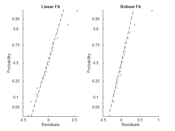
Visually examine the residuals of the two models.
tiledlayout(1,2)
nexttile
plotResiduals(mdl,'probability')
title('Linear Fit')
nexttile
plotResiduals(mdlr,'probability')
title('Robust Fit')

The residuals from the robust fit (right half of the plot) are closer to the straight line, except for the one obvious outlier.
Find the index of the outlier.
outlier = find(isoutlier(mdlr.Residuals.Raw))
outlier =
1
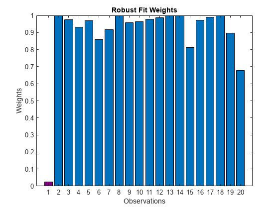
Plot the weights of the observations in the robust fit.
figure
b = bar(mdlr.Robust.Weights);
b.FaceColor = 'flat';
b.CData(outlier,:) = [.5 0 .5];
xticks(1:length(mdlr.Residuals.Raw))
xlabel('Observations')
ylabel('Weights')
title('Robust Fit Weights')

The weight of the outlier in the robust fit (purple bar) is much less than the weights of the other observations.
Steps for Iteratively Reweighted Least Squares
The iteratively reweighted least-squares algorithm follows this procedure:
Start with an initial estimate of the weights and fit the model by weighted least squares.
Compute the adjusted residuals. The adjusted residuals are given by
where ri are the ordinary least-squares residuals, and hi are the least-squares fit leverage values. Leverages adjust the residuals by reducing the weight of high-leverage data points, which have a large effect on the least-squares fit (see Hat Matrix and Leverage).
Standardize the residuals. The standardized adjusted residuals are given by
where K is a tuning constant, and s is an estimate of the standard deviation of the error term given by
s = MAD/0.6745.MADis the median absolute deviation of the residuals from their median. The constant 0.6745 makes the estimate unbiased for the normal distribution. If the predictor data matrixXhas p columns, the software excludes the smallest p absolute deviations when computing the median.Compute the robust weights wi as a function of u. For example, the bisquare weights are given by
Estimate the robust regression coefficients b. The weights modify the expression for the parameter estimates b as follows
where W is the diagonal weight matrix, X is the predictor data matrix, and y is the response vector.
Estimate the weighted least-squares error
where wi are the weights, yi are the observed responses, ŷi are the fitted responses, and ri are the residuals.
Iteration stops if the fit converges or the maximum number of iterations is reached. Otherwise, perform the next iteration of the least-squares fitting by returning to the second step.
See Also
fitlm | robustfit | LinearModel | plotResiduals