ksdensity
Kernel smoothing function estimate for univariate and bivariate data
Syntax
Description
[ returns a probability
density estimate, f,xi]
= ksdensity(x)f, for the sample data in the
vector or two-column matrix x. The estimate is
based on a normal kernel function, and is evaluated at equally-spaced
points, xi, that cover the range of the data
in x. ksdensity estimates
the density at 100 points for univariate data, or 900 points for bivariate
data.
ksdensity works best with continuously
distributed samples.
[
uses additional options specified by one or more name-value pair arguments in
addition to any of the input arguments in the previous syntaxes. For example,
you can define the function type f,xi]
= ksdensity(___,Name,Value)ksdensity evaluates, such
as probability density, cumulative probability, survivor function, and so on. Or
you can specify the bandwidth of the smoothing window.
Examples
Load the sample data.
load carsmall;The variable MPG contains data for car mileage.
Generate a kernel probability density estimate for MPG.
[f,xi] = ksdensity(MPG);
f and xi contain the values and evaluation points for the kernel density estimation. By default, ksdensity uses a normal kernel smoothing function and optimal bandwidth for estimating normal densities.
Plot the estimated density.
plot(xi,f);

The plot shows the pdf of the kernel distribution fit to the MPG data across all makes of cars. The distribution is smooth and slightly skewed with a heavier right tail.
Generate a nonnegative sample data set from the half-normal distribution.
rng('default') % For reproducibility
pd = makedist('HalfNormal','mu',0,'sigma',1);
x = random(pd,100,1);
Estimate pdfs with two different boundary correction methods, log transformation and reflection, by using the 'BoundaryCorrection' name-value pair argument.
pts = linspace(0,5,1000); % points to evaluate the estimator
[f1,xi1] = ksdensity(x,pts,'Support','positive');
[f2,xi2] = ksdensity(x,pts,'Support','positive','BoundaryCorrection','reflection');
Plot the two estimated pdfs.
plot(xi1,f1,xi2,f2)
lgd = legend('log','reflection');
title(lgd, 'Boundary Correction Method')
xl = xlim;
xlim([xl(1)-0.25 xl(2)])
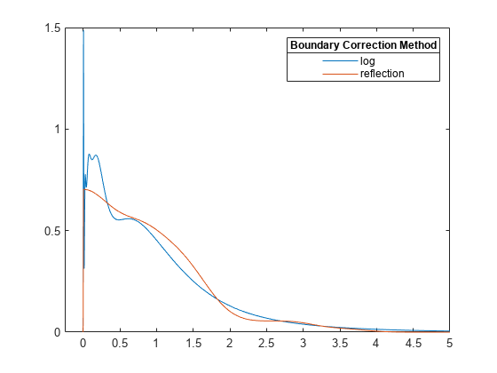
ksdensity uses a boundary correction method when you specify either positive or bounded support. The default boundary correction method is log transformation. When ksdensity transforms the support back, it introduces the 1/x term in the kernel density estimator. Therefore, the estimate has a peak near x = 0. On the other hand, the reflection method does not cause undesirable peaks near the boundary.
Load the sample data.
load hospitalCompute and plot the estimated cdf evaluated at a specified set of values.
pts = (min(hospital.Weight):2:max(hospital.Weight));
figure()
ecdf(hospital.Weight)
hold on
[f,xi,bw] = ksdensity(hospital.Weight,pts,'Support','positive',...
	'Function','cdf');
plot(xi,f,'-g','LineWidth',2)
legend('empirical cdf','kernel-bw:default','Location','northwest')
xlabel('Patient weights')
ylabel('Estimated cdf')

ksdensity seems to smooth the cumulative distribution function estimate too much. An estimate with a smaller bandwidth might produce a closer estimate to the empirical cumulative distribution function.
Return the bandwidth of the smoothing window.
bw
bw =
0.1070
Plot the cumulative distribution function estimate using a smaller bandwidth.
[f,xi] = ksdensity(hospital.Weight,pts,'Support','positive',...
	'Function','cdf','Bandwidth',0.05);
plot(xi,f,'--r','LineWidth',2)
legend('empirical cdf','kernel-bw:default','kernel-bw:0.05',...
	'Location','northwest')
hold off
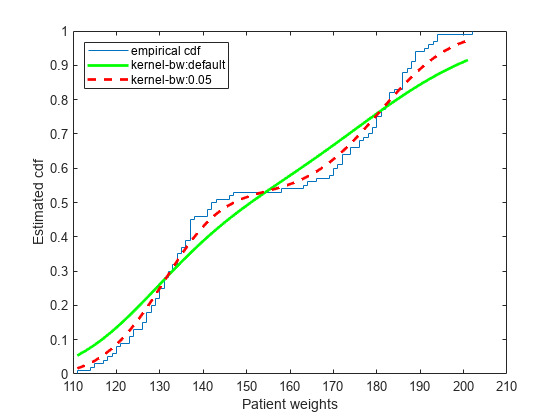
The ksdensity estimate with a smaller bandwidth matches the empirical cumulative distribution function better.
Load the sample data.
load hospitalPlot the estimated cdf evaluated at 50 equally spaced points.
figure()
ksdensity(hospital.Weight,'Support','positive','Function','cdf',...
'NumPoints',50)
xlabel('Patient weights')
ylabel('Estimated cdf')

Generate sample data from an exponential distribution with mean 3.
rng('default')  % For reproducibility
x = random('exp',3,100,1);
Create a logical vector that indicates censoring. Here, observations with lifetimes longer than 10 are censored.
T = 10;
cens = (x>T);
Compute and plot the estimated density function.
figure
ksdensity(x,'Support','positive','Censoring',cens);

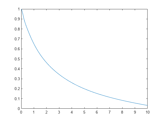
Compute and plot the survivor function.
figure
ksdensity(x,'Support','positive','Censoring',cens,...
'Function','survivor');
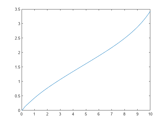
Compute and plot the cumulative hazard function.
figure
ksdensity(x,'Support','positive','Censoring',cens,...
'Function','cumhazard');
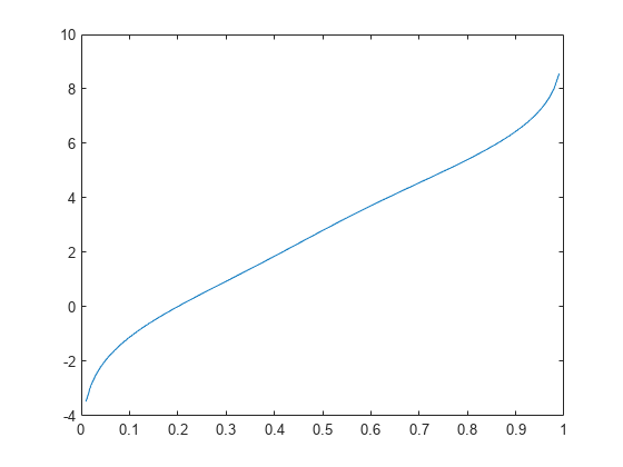
Generate a mixture of two normal distributions, and plot the estimated inverse cumulative distribution function at a specified set of probability values.
rng('default')  % For reproducibility
x = [randn(30,1); 5+randn(30,1)];
pi = linspace(.01,.99,99);
figure
ksdensity(x,pi,'Function','icdf');
Generate a mixture of two normal distributions.
rng('default')  % For reproducibility
x = [randn(30,1); 5+randn(30,1)];
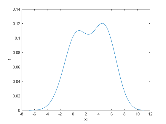
Return the bandwidth of the smoothing window for the probability density estimate.
[f,xi,bw] = ksdensity(x);
bw
bw =
1.5141
The default bandwidth is optimal for normal densities.
Plot the estimated density.
figure
plot(xi,f);
xlabel('xi')
ylabel('f')
hold on
Plot the density using an increased bandwidth value.
[f,xi] = ksdensity(x,'Bandwidth',1.8);
plot(xi,f,'--r','LineWidth',1.5)
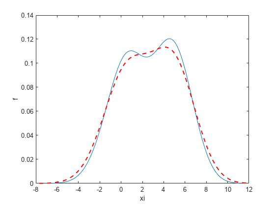
A higher bandwidth further smooths the density estimate, which might mask some characteristics of the distribution.
Now, plot the density using a decreased bandwidth value.
[f,xi] = ksdensity(x,'Bandwidth',0.8);
plot(xi,f,'-.k','LineWidth',1.5)
legend('bw = default','bw = 1.8','bw = 0.8')
hold off
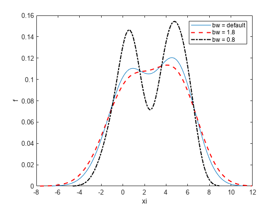
A smaller bandwidth smooths the density estimate less, which exaggerates some characteristics of the sample.
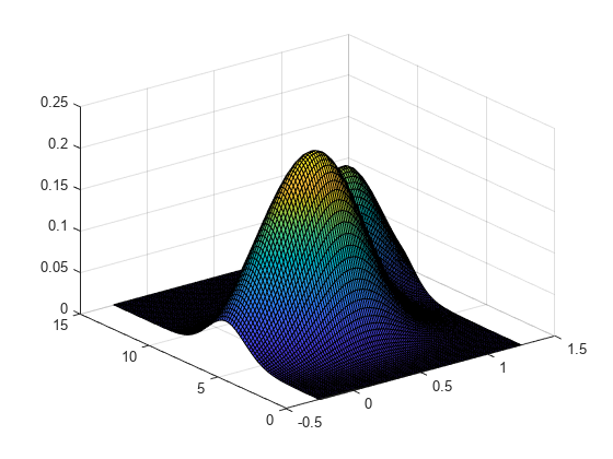
Create a two-column vector of points at which to evaluate the density.
gridx1 = -0.25:.05:1.25;
gridx2 = 0:.1:15;
[x1,x2] = meshgrid(gridx1, gridx2);
x1 = x1(:);
x2 = x2(:);
xi = [x1 x2];
Generate a 30-by-2 matrix containing random numbers from a mixture of bivariate normal distributions.
rng('default')  % For reproducibility
x = [0+.5*rand(20,1) 5+2.5*rand(20,1);
            .75+.25*rand(10,1) 8.75+1.25*rand(10,1)];
Plot the estimated density of the sample data.
figure
ksdensity(x,xi);
Input Arguments
Sample data for which ksdensity returns f values,
specified as a column vector or two-column matrix. Use a column vector
for univariate data, and a two-column matrix for bivariate data.
Example: [f,xi] = ksdensity(x)
Data Types: single | double
Points at which to evaluate f, specified as a vector
or two-column matrix. For univariate data, pts can be a
row or column vector. The length of the returned output
f is equal to the number of points in
pts.
Example: pts = (0:1:25);
ksdensity(x,pts);
Data Types: single | double
Axes handle for the figure ksdensity plots
to, specified as a handle.
For example, if h is a handle for a figure,
then ksdensity can plot to that figure as follows.
Example: ksdensity(h,x)
Name-Value Arguments
Specify optional pairs of arguments as
Name1=Value1,...,NameN=ValueN, where Name is
the argument name and Value is the corresponding value.
Name-value arguments must appear after other arguments, but the order of the
pairs does not matter.
Before R2021a, use commas to separate each name and value, and enclose
Name in quotes.
Example: 'Censoring',cens,'Kernel','triangle','NumPoints',20,'Function','cdf'
specifies that ksdensity estimates the cdf by evaluating at 20
equally spaced points that covers the range of data, using the triangle kernel
smoothing function and accounting for the censored data information in vector
cens.
Bandwidth of the kernel smoothing window, which is a function of the
number of points in x, specified as
"normal-approx" or "plug-in".
If the sample data is bivariate, Bandwidth can also
be a two-element vector [L,U].
When
Bandwidthis"normal-approx",ksdensityuses the normal approximation method, or Silverman's rule of thumb, to calculate the bandwidth. The calculated value is optimal for estimating normal densities [2], but you might want to specify a larger value for more smoothing or a smaller value for less.When
Bandwidthis"plug-in",ksdensityuses the improved plug-in method described in [1] to calculate the bandwidth. The plug-in method is sometimes called the Sheather-Jones method.When
Bandwidthis a positive scalar, its value controls the smoothness of the probability function estimate. As the value increases, the probability function estimate gets smoother.
If you specify BoundaryCorrection as
"log"(default) and Support
as either "positive" or a vector [L
U], ksdensity converts bounded data
to unbounded by using log transformation. The value of
Bandwidth is on the scale of the transformed
values.
Example: Bandwidth=0.8
Data Types: single | double
Boundary correction method, specified as the comma-separated pair
consisting of 'BoundaryCorrection' and
'log' or 'reflection'.
| Value | Description |
|---|---|
'log' |
The value of |
'reflection' |
|
ksdensity applies boundary correction only when
you specify 'Support' as a value other than
'unbounded'.
Example: 'BoundaryCorrection','reflection'
Logical vector indicating which entries are censored, specified as the
comma-separated pair consisting of 'Censoring' and a
vector of binary values. A value of 0 indicates there is no censoring, 1
indicates that observation is censored. Default is there is no
censoring. This name-value pair is only valid for univariate
data.
Example: 'Censoring',censdata
Data Types: logical
Function to estimate, specified as the comma-separated pair consisting
of 'Function' and one of the following.
| Value | Description |
|---|---|
'pdf' | Probability density function. |
'cdf' | Cumulative distribution function. |
'icdf' |
Inverse cumulative distribution function.
This value is valid only for univariate data. |
'survivor' | Survivor function. |
'cumhazard' |
Cumulative hazard function. This value is valid only for univariate data. |
Example: 'Function','icdf'
Type of kernel smoother, specified as the comma-separated pair
consisting of 'Kernel' and one of the
following.
'normal'(default)'box''triangle''epanechnikov'A kernel function that is a custom or built-in function. Specify the function as a function handle (for example,
@myfunctionor@normpdf) or as a character vector or string scalar (for example,'myfunction'or'normpdf'). The software calls the specified function with one argument that is an array of distances between data values and locations where the density is evaluated. The function must return an array of the same size containing corresponding values of the kernel function.When
'Function'is'pdf', the kernel function returns density values. Otherwise, it returns cumulative probability values.Specifying a custom kernel when
'Function'is'icdf'returns an error.
For bivariate data, ksdensity applies the same
kernel to each dimension.
Example: 'Kernel','box'
Number of equally spaced points in xi, specified
as the comma-separated pair consisting of 'NumPoints'
and a scalar value. This name-value pair is only valid for univariate
data.
For example, for a kernel smooth estimate of a specified function at 80 equally spaced points within the range of sample data, input:
Example: 'NumPoints',80
Data Types: single | double
Support for the density, specified as one of the following values.
| Value | Description |
|---|---|
"unbounded" | Allow the density to extend over the whole real line (default). |
"positive" | Restrict the density to positive values. |
"nonnegative" | Restrict the density to positive values and
0. |
"negative" | Restrict the density to negative values. |
Two-element vector [L U] | Give the finite lower and upper bounds for the support of the density. This option is valid only for univariate sample data. |
Two-by-two matrix [L1 L2; U1
U2] | Give the finite lower and upper bounds for the support of the density. The first row contains the lower limits, and the second row contains the upper limits. This option is valid only for bivariate sample data. |
For bivariate data, Support can be a combination of
positive, unbounded, and bounded variables specified as [0
-Inf; Inf Inf] or [0 L; Inf U].
Example: Support="positive"
Example: Support=[0 10]
Data Types: single | double | char | string
Function used to create kernel density plot, specified as the
comma-separated pair consisting of 'PlotFcn' and one
of the following.
| Value | Description |
|---|---|
'surf' | 3-D shaded surface plot, created using surf |
'contour' | Contour plot, created using contour |
'plot3' | 3-D line plot, created using plot3 |
'surfc' | Contour plot under a 3-D shaded surface plot, created
using surfc |
This name-value pair is only valid for bivariate sample data.
Example: 'PlotFcn','contour'
Weights for sample data, specified as the comma-separated pair consisting of
'Weights' and a vector of length size(x,1),
where x is the sample data.
Example: 'Weights',xw
Data Types: single | double
Output Arguments
Evaluation points at which ksdensity calculates f,
returned as a vector or a two-column matrix. For univariate data, the
default is 100 equally-spaced points that cover the range of data in
x. For bivariate data, the default is 900
equally-spaced points created using meshgrid from 30
equally-spaced points in each dimension.
Bandwidth of smoothing window, returned as a scalar value.
If you specify 'BoundaryCorrection' as
'log'(default) and 'Support' as
either 'positive' or a vector [L U],
ksdensity converts bounded data to be unbounded by
using log transformation. The value of bw is on the
scale of the transformed values.
More About
A kernel distribution is a nonparametric representation of the probability density function (pdf) of a random variable. You can use a kernel distribution when a parametric distribution cannot properly describe the data, or when you want to avoid making assumptions about the distribution of the data. A kernel distribution is defined by a smoothing function and a bandwidth value, which control the smoothness of the resulting density curve.
The kernel density estimator is the estimated pdf of a random variable. For any real values of x, the kernel density estimator's formula is given by
where x1, x2, …, xn are random samples from an unknown distribution, n is the sample size, is the kernel smoothing function, and h is the bandwidth.
The kernel estimator for the cumulative distribution function (cdf), for any real values of x, is given by
where .
For more details, see Kernel Distribution.
The reflection method is a boundary correction method that
accurately finds kernel density estimators when a random variable has bounded
support. If you specify 'BoundaryCorrection','reflection',
ksdensity uses the reflection method. This method augments
bounded data by adding reflected data near the boundaries, and estimates the pdf.
Then, ksdensity returns the estimated pdf corresponding to the
original support with proper normalization, so that the estimated pdf's integral
over the original support is equal to one.
If you additionally specify 'Support',[L U], then
ksdensity finds the kernel estimator as follows.
If
'Function'is'pdf', then the kernel density estimator isfor L ≤ x ≤ U,
where , , and xi is the
ith sample data.If
'Function'is'cdf', then the kernel estimator for cdf isfor L ≤ x ≤ U.
To obtain a kernel estimator for an inverse cdf, a survivor function, or a cumulative hazard function (when
'Function'is'icdf','survivor', or'cumhazrd'),ksdensityuses both and .
If you additionally specify 'Support' as
'positive' or [0 inf], then
ksdensity finds the kernel estimator by replacing
[L U] with [0 inf] in the above
equations.
Alternative Functionality
You can also estimate the pdf or cdf for univariate data by using the MATLAB®
kde
function. Unlike ksdensity, kde does not
support boundary correction methods or data censoring.
References
[1] Botev, Z. I., J. F. Grotowski, and D. P. Kroese. "Kernel Density Estimation via Diffusion." The Annals of Statistics, vol. 38, no. 5 (October 1, 2010). https://projecteuclid.org/journals/annals-of-statistics/volume-38/issue-5/Kernel-density-estimation-via-diffusion/10.1214/10-AOS799.full
[2] Bowman, A. W., and A. Azzalini. Applied Smoothing Techniques for Data Analysis. New York: Oxford University Press Inc., 1997.
[3] Hill, P. D. “Kernel estimation of a distribution function.” Communications in Statistics - Theory and Methods. Vol 14, Issue. 3, 1985, pp. 605-620.
[4] Jones, M. C. “Simple boundary correction for kernel density estimation.” Statistics and Computing. Vol. 3, Issue 3, 1993, pp. 135-146.
[5] Silverman, B. W. Density Estimation for Statistics and Data Analysis. Chapman & Hall/CRC, 1986.
Extended Capabilities
This function supports tall arrays for out-of-memory data with some limitations.
Some options that require extra passes or sorting of the input data are not supported:
'BoundaryCorrection''Censoring''Support'(support is always unbounded).
Uses standard deviation (instead of median absolute deviation) to compute the bandwidth.
For more information, see Tall Arrays for Out-of-Memory Data.
Usage notes and limitations:
Plotting is not supported.
Names in name-value pair arguments must be compile-time constants.
Values in the following name-value pair arguments must also be compile-time constants:
'BoundaryCorrection','Function', and'Kernel'. For example, to use the'Function','cdf'name-value pair argument in the generated code, include{coder.Constant('Function'),coder.Constant('cdf')}in the-argsvalue ofcodegen.The value of the
'Kernel'name-value pair argument cannot be a custom function handle. To specify a custom kernel function, use a character vector or string scalar.For the value of the
'Support'name-value pair argument, the compile-time data type must match the runtime data type.
For more information on code generation, see Introduction to Code Generation for Statistics and Machine Learning Functions and Overview of Code Generation Using MATLAB Coder (MATLAB Coder).
This function fully supports GPU arrays. For more information, see Run MATLAB Functions on a GPU (Parallel Computing Toolbox).
Version History
Introduced before R2006a
MATLAB Command
You clicked a link that corresponds to this MATLAB command:
Run the command by entering it in the MATLAB Command Window. Web browsers do not support MATLAB commands.
Select a Web Site
Choose a web site to get translated content where available and see local events and offers. Based on your location, we recommend that you select: .
You can also select a web site from the following list
How to Get Best Site Performance
Select the China site (in Chinese or English) for best site performance. Other MathWorks country sites are not optimized for visits from your location.
Americas
- América Latina (Español)
- Canada (English)
- United States (English)
Europe
- Belgium (English)
- Denmark (English)
- Deutschland (Deutsch)
- España (Español)
- Finland (English)
- France (Français)
- Ireland (English)
- Italia (Italiano)
- Luxembourg (English)
- Netherlands (English)
- Norway (English)
- Österreich (Deutsch)
- Portugal (English)
- Sweden (English)
- Switzerland
- United Kingdom (English)