incrementalLearner

Convert kernel model for binary classification to incremental learner

Since R2022a

Syntax

IncrementalMdl = incrementalLearner(Mdl)

IncrementalMdl = incrementalLearner(Mdl,Name=Value)

Description

IncrementalMdl = incrementalLearner(Mdl) returns a binary Gaussian kernel classification model for incremental learning, IncrementalMdl, using the traditionally trained kernel model object or kernel model template object in Mdl.

If you specify a traditionally trained model, then its property values reflect the knowledge gained from Mdl (parameters and hyperparameters of the model). Therefore, IncrementalMdl can predict labels given new observations, and it is warm, meaning that its predictive performance is tracked.

IncrementalMdl = incrementalLearner(Mdl,Name=Value) uses additional options specified by one or more name-value arguments. Some options require you to train IncrementalMdl before its predictive performance is tracked. For example, MetricsWarmupPeriod=50,MetricsWindowSize=100 specifies a preliminary incremental training period of 50 observations before performance metrics are tracked, and specifies processing 100 observations before updating the window performance metrics.

Examples

Convert Traditionally Trained Model to Incremental Learner

Train a kernel classification model for binary learning by using fitckernel, and then convert it to an incremental learner.

Load and Preprocess Data

Load the human activity data set.

load humanactivity

For details on the data set, enter Description at the command line.

Responses can be one of five classes: Sitting, Standing, Walking, Running, or Dancing. Dichotomize the response by identifying whether the subject is moving (actid > 2).

Y = actid > 2;

Train Kernel Classification Model

Fit a kernel classification model to the entire data set.

Mdl = fitckernel(feat,Y)

Mdl = 
  ClassificationKernel
              ResponseName: 'Y'
                ClassNames: [0 1]
                   Learner: 'svm'
    NumExpansionDimensions: 2048
               KernelScale: 1
                    Lambda: 4.1537e-05
             BoxConstraint: 1


  Properties, Methods

Mdl is a ClassificationKernel model object representing a traditionally trained kernel classification model.

Convert Trained Model

Convert the traditionally trained kernel classification model to a model for incremental learning.

IncrementalMdl = incrementalLearner(Mdl,Solver="sgd",LearnRate=1)

IncrementalMdl = 
  incrementalClassificationKernel

                    IsWarm: 1
                   Metrics: [1x2 table]
                ClassNames: [0 1]
            ScoreTransform: 'none'
    NumExpansionDimensions: 2048
               KernelScale: 1


  Properties, Methods

IncrementalMdl is an incrementalClassificationKernel model object prepared for incremental learning.

• The incrementalLearner function initializes the incremental learner by passing model parameters to it, along with other information Mdl extracted from the training data.

• IncrementalMdl is warm (IsWarm is 1), which means that incremental learning functions can start tracking performance metrics.

• incrementalClassificationKernel trains the model using the adaptive scale-invariant solver, whereas fitckernel trained Mdl using the Limited-memory Broyden-Fletcher-Goldfarb-Shanno (LBFGS) solver.

Predict Responses

An incremental learner created from converting a traditionally trained model can generate predictions without further processing.

Predict classification scores for all observations using both models.

[~,ttscores] = predict(Mdl,feat);
[~,ilscores] = predict(IncrementalMdl,feat);
compareScores = norm(ttscores(:,1) - ilscores(:,1))

compareScores = 0

The difference between the scores generated by the models is 0.

Configure Performance Metric Options

Use a trained kernel classification model to initialize an incremental learner. Prepare the incremental learner by specifying a metrics warm-up period and a metrics window size.

Load the human activity data set.

load humanactivity

For details on the data set, enter Description at the command line.

Responses can be one of five classes: Sitting, Standing, Walking, Running, and Dancing. Dichotomize the response by identifying whether the subject is moving (actid > 2).

Y = actid > 2;

Because the data set is grouped by activity, shuffle it for simplicity. Then, randomly split the data in half: the first half for training a model traditionally, and the second half for incremental learning.

n = numel(Y);

rng(1) % For reproducibility
cvp = cvpartition(n,Holdout=0.5);
idxtt = training(cvp);
idxil = test(cvp);
shuffidx = randperm(n);
X = feat(shuffidx,:);
Y = Y(shuffidx);

% First half of data
Xtt = X(idxtt,:);
Ytt = Y(idxtt);

% Second half of data
Xil = X(idxil,:);
Yil = Y(idxil);

Fit a kernel classification model to the first half of the data.

Mdl = fitckernel(Xtt,Ytt);

Convert the traditionally trained kernel classification model to a model for incremental learning. Specify the following:

• A performance metrics warm-up period of 2000 observations

• A metrics window size of 500 observations

• Use of classification error and hinge loss to measure the performance of the model

IncrementalMdl = incrementalLearner(Mdl, ...
    MetricsWarmupPeriod=2000,MetricsWindowSize=500, ...
    Metrics=["classiferror","hinge"]);

Fit the incremental model to the second half of the data by using the updateMetricsAndFit function. At each iteration:

• Simulate a data stream by processing 20 observations at a time.

• Overwrite the previous incremental model with a new one fitted to the incoming observations.

• Store the cumulative metrics, window metrics, and number of training observations to see how they evolve during incremental learning.

% Preallocation
nil = numel(Yil);
numObsPerChunk = 20;
nchunk = ceil(nil/numObsPerChunk);
ce = array2table(zeros(nchunk,2),VariableNames=["Cumulative","Window"]);
hinge = array2table(zeros(nchunk,2),VariableNames=["Cumulative","Window"]); 
numtrainobs = [zeros(nchunk,1)];

% Incremental fitting
for j = 1:nchunk
    ibegin = min(nil,numObsPerChunk*(j-1) + 1);
    iend   = min(nil,numObsPerChunk*j);
    idx = ibegin:iend;    
    IncrementalMdl = updateMetricsAndFit(IncrementalMdl,Xil(idx,:),Yil(idx));
    ce{j,:} = IncrementalMdl.Metrics{"ClassificationError",:};
    hinge{j,:} = IncrementalMdl.Metrics{"HingeLoss",:};
    numtrainobs(j) = IncrementalMdl.NumTrainingObservations;
end

IncrementalMdl is an incrementalClassificationKernel model object trained on all the data in the stream. During incremental learning and after the model is warmed up, updateMetricsAndFit checks the performance of the model on the incoming observations, and then fits the model to those observations.

Plot a trace plot of the number of training observations and the performance metrics on separate tiles.

t = tiledlayout(3,1);
nexttile
plot(numtrainobs)
xlim([0 nchunk])
ylabel(["Number of","Training Observations"])
xline(IncrementalMdl.MetricsWarmupPeriod/numObsPerChunk,"--")
nexttile
plot(ce.Variables)
xlim([0 nchunk])
ylabel("Classification Error")
xline(IncrementalMdl.MetricsWarmupPeriod/numObsPerChunk,"--")
legend(ce.Properties.VariableNames,Location="best")
nexttile
plot(hinge.Variables)
xlim([0 nchunk])
ylabel("Hinge Loss")
xline(IncrementalMdl.MetricsWarmupPeriod/numObsPerChunk,"--")
xlabel(t,"Iteration")

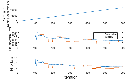
The plot suggests that updateMetricsAndFit does the following:

• Fit the model during all incremental learning iterations.

• Compute the performance metrics after the metrics warm-up period only.

• Compute the cumulative metrics during each iteration.

• Compute the window metrics after processing 500 observations (25 iterations).

Specify SGD Solver

The default solver for incrementalClassificationKernel is the adaptive scale-invariant solver, which does not require hyperparameter tuning before you fit a model. However, if you specify either the standard stochastic gradient descent (SGD) or average SGD (ASGD) solver instead, you can also specify an estimation period, during which the incremental fitting functions tune the learning rate.

Load the human activity data set.

load humanactivity

For details on the data set, enter Description at the command line.

Responses can be one of five classes: Sitting, Standing, Walking, Running, and Dancing. Dichotomize the response by identifying whether the subject is moving (actid > 2).

Y = actid > 2;

Randomly split the data in half: the first half for training a model traditionally, and the second half for incremental learning.

n = numel(Y);

rng(1) % For reproducibility
cvp = cvpartition(n,Holdout=0.5);
idxtt = training(cvp);
idxil = test(cvp);

% First half of data 
Xtt = feat(idxtt,:);
Ytt = Y(idxtt);

% Second half of data
Xil = feat(idxil,:);
Yil = Y(idxil);

Fit a kernel classification model to the first half of the data.

TTMdl = fitckernel(Xtt,Ytt);

Convert the traditionally trained kernel classification model to a model for incremental learning. Specify the standard SGD solver and an estimation period of 2000 observations (the default is 1000 when a learning rate is required).

IncrementalMdl = incrementalLearner(TTMdl,Solver="sgd",EstimationPeriod=2000);

IncrementalMdl is an incrementalClassificationKernel model object configured for incremental learning.

Fit the incremental model to the second half of the data by using the fit function. At each iteration:

• Simulate a data stream by processing 10 observations at a time.

• Overwrite the previous incremental model with a new one fitted to the incoming observations.

• Store the initial learning rate and number of training observations to see how they evolve during training.

% Preallocation
nil = numel(Yil);
numObsPerChunk = 10;
nchunk = floor(nil/numObsPerChunk);
learnrate = [zeros(nchunk,1)];
numtrainobs = [zeros(nchunk,1)];

% Incremental fitting
for j = 1:nchunk
    ibegin = min(nil,numObsPerChunk*(j-1) + 1);
    iend   = min(nil,numObsPerChunk*j);
    idx = ibegin:iend;
    IncrementalMdl = fit(IncrementalMdl,Xil(idx,:),Yil(idx));
    learnrate(j) = IncrementalMdl.SolverOptions.LearnRate;
    numtrainobs(j) = IncrementalMdl.NumTrainingObservations;
end

IncrementalMdl is an incrementalClassificationKernel model object trained on all the data in the stream.

Plot a trace plot of the number of training observations and the initial learning rate on separate tiles.

t = tiledlayout(2,1);
nexttile
plot(numtrainobs)
xlim([0 nchunk])
xline(IncrementalMdl.EstimationPeriod/numObsPerChunk,"-.");
ylabel("Number of Training Observations")
nexttile
plot(learnrate)
xlim([0 nchunk])
ylabel("Initial Learning Rate")
xline(IncrementalMdl.EstimationPeriod/numObsPerChunk,"-.");
xlabel(t,"Iteration")

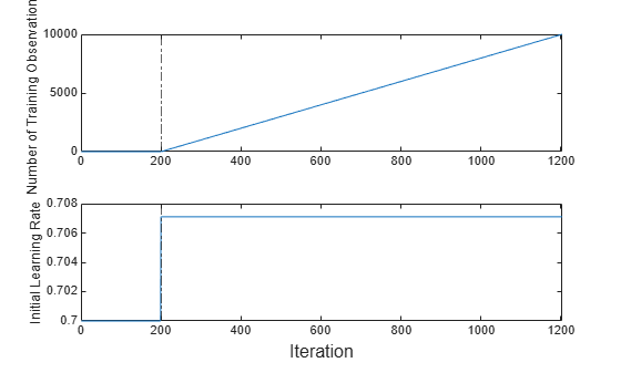
The plot suggests that the fit function does not fit the model to the streaming data during the estimation period. The initial learning rate jumps from 0.7 to its autotuned value after the estimation period. During training, the software uses a learning rate that gradually decays from the initial value specified in the LearnRateSchedule property of IncrementalMdl.

Input Arguments

Mdl — Traditionally trained model or model template

ClassificationKernel model object | kernel model template

Traditionally trained Gaussian kernel model or kernel model template, specified as a ClassificationKernel model object returned by fitckernel or a template object returned by templateKernel, respectively.

Note

Incremental learning functions support only numeric input predictor data. If Mdl was trained on categorical data, you must prepare an encoded version of the categorical data to use incremental learning functions. Use dummyvar to convert each categorical variable to a numeric matrix of dummy variables. Then, concatenate all dummy variable matrices and any other numeric predictors, in the same way that the training function encodes categorical data. For more details, see Dummy Variables.

Name-Value Arguments

Specify optional pairs of arguments as Name1=Value1,...,NameN=ValueN, where Name is the argument name and Value is the corresponding value. Name-value arguments must appear after other arguments, but the order of the pairs does not matter.

Example: Solver="sgd",MetricsWindowSize=100 specifies the stochastic gradient descent solver for objective optimization, and specifies processing 100 observations before updating the window performance metrics.

General Options

Solver — Objective function minimization technique

"scale-invariant" (default) | "sgd" | "asgd"

Objective function minimization technique, specified as a value in this table.

Value	Description	Notes
"scale-invariant"	Adaptive scale-invariant solver for incremental learning [1]	This algorithm is parameter free and can adapt to differences in predictor scales. Try this algorithm before using SGD or ASGD. To shuffle an incoming chunk of data before the fit function fits the model, set Shuffle to true.
"sgd"	Stochastic gradient descent (SGD) [2][3]	To train effectively with SGD, specify adequate values for hyperparameters using options listed in SGD and ASGD Solver Options. The fit function always shuffles an incoming chunk of data before fitting the model.
"asgd"	Average stochastic gradient descent (ASGD) [4]	To train effectively with ASGD, specify adequate values for hyperparameters using options listed in SGD and ASGD Solver Options. The fit function always shuffles an incoming chunk of data before fitting the model.

Example: Solver="sgd"

Data Types: char | string

EstimationPeriod — Number of observations processed to estimate hyperparameters

nonnegative integer

Number of observations processed by the incremental model to estimate hyperparameters before training or tracking performance metrics, specified as a nonnegative integer.

Note

• If Mdl is prepared for incremental learning (all hyperparameters required for training are specified), incrementalLearner forces EstimationPeriod to 0.

• If Mdl is not prepared for incremental learning, incrementalLearner sets EstimationPeriod to 1000.

For more details, see Estimation Period.

Example: EstimationPeriod=100

Data Types: single | double

SGD and ASGD Solver Options

BatchSize — Mini-batch size

10 (default) | positive integer

Mini-batch size, specified as a positive integer. At each learning cycle during training, incrementalLearner uses BatchSize observations to compute the subgradient.

The number of observations in the last mini-batch (last learning cycle in each function call of fit or updateMetricsAndFit) can be smaller than BatchSize. For example, if you supply 25 observations to fit or updateMetricsAndFit, the function uses 10 observations for the first two learning cycles and 5 observations for the last learning cycle.

Example: BatchSize=5

Data Types: single | double

Lambda — Ridge (L2) regularization term strength

1e-5 (default) | nonnegative scalar

Ridge (L2) regularization term strength, specified as a nonnegative scalar.

Example: Lambda=0.01

Data Types: single | double

LearnRate — Initial learning rate

"auto" (default) | positive scalar

Initial learning rate, specified as "auto" or a positive scalar.

The learning rate controls the optimization step size by scaling the objective subgradient. LearnRate specifies an initial value for the learning rate, and LearnRateSchedule determines the learning rate for subsequent learning cycles.

When you specify "auto":

• The initial learning rate is 0.7.

• If EstimationPeriod > 0, fit and updateMetricsAndFit change the rate to 1/sqrt(1+max(sum(X.^2,2))) at the end of EstimationPeriod.

Example: LearnRate=0.001

Data Types: single | double | char | string

LearnRateSchedule — Learning rate schedule

"decaying" (default) | "constant"

Learning rate schedule, specified as a value in this table, where LearnRate specifies the initial learning rate ɣ₀.

Value	Description
"constant"	The learning rate is ɣ0 for all learning cycles.
"decaying"	The learning rate at learning cycle t is $${\gamma }_t=\frac{{\gamma }_0}{{\left(1+\lambda {\gamma }_{0}t\right)}^c}.$$ λ is the value of Lambda. If Solver is "sgd", then c = 1. If Solver is "asgd", then c = 0.75 [4].

Example: LearnRateSchedule="constant"

Data Types: char | string

Adaptive Scale-Invariant Solver Options

Shuffle — Flag for shuffling observations

true or 1 (default) | false or 0

Flag for shuffling the observations at each iteration, specified as logical 1 (true) or 0 (false).

Value	Description
logical 1 (true)	The software shuffles the observations in an incoming chunk of data before the fit function fits the model. This action reduces bias induced by the sampling scheme.
logical 0 (false)	The software processes the data in the order received.

Example: Shuffle=false

Data Types: logical

Performance Metrics Options

Metrics — Model performance metrics to track during incremental learning

"classiferror" (default) | string vector | function handle | cell vector | structure array | "binodeviance" | "exponential" | "hinge" | "logit" | "quadratic"

Model performance metrics to track during incremental learning with the updateMetrics or updateMetricsAndFit function, specified as a built-in loss function name, string vector of names, function handle (@metricName), structure array of function handles, or cell vector of names, function handles, or structure arrays.

The following table lists the built-in loss function names. You can specify more than one by using a string vector.

Name	Description
"binodeviance"	Binomial deviance
"classiferror"	Classification error
"exponential"	Exponential loss
"hinge"	Hinge loss
"logit"	Logistic loss
"quadratic"	Quadratic loss

For more details on the built-in loss functions, see loss.

Example: Metrics=["classiferror","hinge"]

To specify a custom function that returns a performance metric, use function handle notation. The function must have this form:

metric = customMetric(C,S)

• The output argument metric is an n-by-1 numeric vector, where each element is the loss of the corresponding observation in the data processed by the incremental learning functions during a learning cycle.

• You specify the function name (customMetric).

• C is an n-by-2 logical matrix with rows indicating the class to which the corresponding observation belongs. The column order corresponds to the class order in the model for incremental learning. Create C by setting C(p,q) = 1, if observation p is in class q, for each observation in the specified data. Set the other element in row p to 0.

• S is an n-by-2 numeric matrix of predicted classification scores. S is similar to the score output of predict, where rows correspond to observations in the data and the column order corresponds to the class order in the model for incremental learning. S(p,q) is the classification score of observation p being classified in class q.

To specify multiple custom metrics and assign a custom name to each, use a structure array. To specify a combination of built-in and custom metrics, use a cell vector.

Example: Metrics=struct(Metric1=@customMetric1,Metric2=@customMetric2)

Example: Metrics={@customMetric1,@customMetric2,"logit",struct(Metric3=@customMetric3)}

updateMetrics and updateMetricsAndFit store specified metrics in a table in the property IncrementalMdl.Metrics. The data type of Metrics determines the row names of the table.

Metrics Value Data Type	Description of Metrics Property Row Name	Example
String or character vector	Name of corresponding built-in metric	Row name for "classiferror" is "ClassificationError"
Structure array	Field name	Row name for struct(Metric1=@customMetric1) is "Metric1"
Function handle to function stored in a program file	Name of function	Row name for @customMetric is "customMetric"
Anonymous function	CustomMetric_j, where j is metric j in Metrics	Row name for @(C,S)customMetric(C,S)... is CustomMetric_1

For more details on performance metrics options, see Performance Metrics.

Data Types: char | string | struct | cell | function_handle

MetricsWarmupPeriod — Number of observations fit before tracking performance metrics

0 (default) | nonnegative integer

Number of observations the incremental model must be fit to before it tracks performance metrics in its Metrics property, specified as a nonnegative integer. The incremental model is warm after incremental fitting functions fit (EstimationPeriod + MetricsWarmupPeriod) observations to the incremental model.

For more details on performance metrics options, see Performance Metrics.

Example: MetricsWarmupPeriod=50

Data Types: single | double

MetricsWindowSize — Number of observations to use to compute window performance metrics

200 (default) | positive integer

Number of observations to use to compute window performance metrics, specified as a positive integer.

For more details on performance metrics options, see Performance Metrics.

Example: MetricsWindowSize=250

Data Types: single | double

Output Arguments

IncrementalMdl — Binary Gaussian kernel classification model for incremental learning

incrementalClassificationKernel model object

Binary Gaussian kernel classification model for incremental learning, returned as an incrementalClassificationKernel model object. IncrementalMdl is also configured to generate predictions given new data (see predict).

The incrementalLearner function initializes IncrementalMdl for incremental learning using the model information in Mdl. The following table shows the Mdl properties that incrementalLearner passes to corresponding properties of IncrementalMdl. The function also passes other model information required to initialize IncrementalMdl, such as learned model coefficients, regularization term strength, and the random number stream.

Input Object Mdl Type	Property	Description
ClassificationKernel model object or kernel model template object	KernelScale	Kernel scale parameter, a positive scalar
	Learner	Linear classification model type, a character vector
	NumExpansionDimensions	Number of dimensions of expanded space, a positive integer
ClassificationKernel model object	ClassNames	Class labels for binary classification, a two-element list
	NumPredictors	Number of predictors, a positive integer
	Prior	Prior class label distribution, a numeric vector
	ScoreTransform	Score transformation function, a function name or function handle

Note that incrementalLearner does not use the Cost property of the traditionally trained model in Mdl because incrementalClassificationKernel does not support this property.

More About

Incremental Learning

Incremental learning, or online learning, is a branch of machine learning concerned with processing incoming data from a data stream, possibly given little to no knowledge of the distribution of the predictor variables, aspects of the prediction or objective function (including tuning parameter values), or whether the observations are labeled. Incremental learning differs from traditional machine learning, where enough labeled data is available to fit to a model, perform cross-validation to tune hyperparameters, and infer the predictor distribution.

Given incoming observations, an incremental learning model processes data in any of the following ways, but usually in this order:

• Predict labels.

• Measure the predictive performance.

• Check for structural breaks or drift in the model.

• Fit the model to the incoming observations.

For more details, see Incremental Learning Overview.

Adaptive Scale-Invariant Solver for Incremental Learning

The adaptive scale-invariant solver for incremental learning, introduced in [1], is a gradient-descent-based objective solver for training linear predictive models. The solver is hyperparameter free, insensitive to differences in predictor variable scales, and does not require prior knowledge of the distribution of the predictor variables. These characteristics make it well suited to incremental learning.

The incremental fitting functions fit and updateMetricsAndFit use the more aggressive ScInOL2 version of the algorithm.

Random Feature Expansion

Random feature expansion, such as Random Kitchen Sinks[5] or Fastfood[6], is a scheme to approximate Gaussian kernels of the kernel classification algorithm to use for big data in a computationally efficient way. Random feature expansion is more practical for big data applications that have large training sets, but can also be applied to smaller data sets that fit in memory.

The kernel classification algorithm searches for an optimal hyperplane that separates the data into two classes after mapping features into a high-dimensional space. Nonlinear features that are not linearly separable in a low-dimensional space can be separable in the expanded high-dimensional space. All the calculations for hyperplane classification use only dot products. You can obtain a nonlinear classification model by replacing the dot product x₁x₂' with the nonlinear kernel function $$G(x_1,x_2)=\langle \phi (x_1),\phi (x_2)\rangle$$, where x_i is the ith observation (row vector) and φ(x_i) is a transformation that maps x_i to a high-dimensional space (called the “kernel trick”). However, evaluating G(x₁,x₂) (Gram matrix) for each pair of observations is computationally expensive for a large data set (large n).

The random feature expansion scheme finds a random transformation so that its dot product approximates the Gaussian kernel. That is,

$$G(x_1,x_2)=\langle \phi (x_1),\phi (x_2)\rangle \approx T(x_1)T(x_2)\text{'},$$

where T(x) maps x in $${ℝ}^p$$ to a high-dimensional space ($${ℝ}^m$$). The Random Kitchen Sinks scheme uses the random transformation

$$T(x)=m^{-1/2}\exp \left(iZx\text{'}\right)\text{'},$$

where $$Z\in {ℝ}^{m\times p}$$ is a sample drawn from $$N\left(0,{\sigma }^{-2}\right)$$ and σ is a kernel scale. This scheme requires O(mp) computation and storage.

The Fastfood scheme introduces another random basis V instead of Z using Hadamard matrices combined with Gaussian scaling matrices. This random basis reduces the computation cost to O(mlogp) and reduces storage to O(m).

incrementalClassificationKernel uses the Fastfood scheme for random feature expansion, and uses linear classification to train a Gaussian kernel classification model. You can specify values for m and σ using the NumExpansionDimensions and KernelScale name-value arguments, respectively, when you create a traditionally trained model using fitckernel or when you callincrementalClassificationKernel directly to create the model object.

Algorithms

Estimation Period

During the estimation period, the incremental fitting functions fit and updateMetricsAndFit use the first incoming EstimationPeriod observations to estimate (tune) hyperparameters required for incremental training. Estimation occurs only when EstimationPeriod is positive. This table describes the hyperparameters and when they are estimated, or tuned.

Hyperparameter	Model Property	Usage	Conditions
Learning rate	LearnRate field of SolverOptions	Adjust the solver step size	The hyperparameter is estimated when both of these conditions apply: You specify the Solver name-value argument as "sgd" or "asgd". You do not specify the LearnRate name-value argument as a positive scalar.
Kernel scale parameter	KernelScale	Set a kernel scale parameter value for random feature expansion	The software does not estimate KernelScale if you create an incrementalClassificationKernel model object by using incrementalLearner. If you create an incrementalClassificationKernel model object by calling the incrementalClassificationKernel function, the software estimates KernelScale in some cases. For details, see Estimation Period on the incrementalClassificationKernel page.

During the estimation period, fit does not fit the model, and updateMetricsAndFit does not fit the model or update the performance metrics. At the end of the estimation period, the functions update the properties that store the hyperparameters.

Performance Metrics

• The updateMetrics and updateMetricsAndFit functions are incremental learning functions that track model performance metrics (Metrics) from new data only when the incremental model is warm (IsWarm property is true). An incremental model becomes warm after fit or updateMetricsAndFit fits the incremental model to MetricsWarmupPeriod observations, which is the metrics warm-up period.

  If EstimationPeriod > 0, the fit and updateMetricsAndFit functions estimate hyperparameters before fitting the model to data. Therefore, the functions must process an additional EstimationPeriod observations before the model starts the metrics warm-up period.

• The Metrics property of the incremental model stores two forms of each performance metric as variables (columns) of a table, Cumulative and Window, with individual metrics in rows. When the incremental model is warm, updateMetrics and updateMetricsAndFit update the metrics at the following frequencies:

  • Cumulative — The functions compute cumulative metrics since the start of model performance tracking. The functions update metrics every time you call the functions and base the calculation on the entire supplied data set.

  • Window — The functions compute metrics based on all observations within a window determined by MetricsWindowSize, which also determines the frequency at which the software updates Window metrics. For example, if MetricsWindowSize is 20, the functions compute metrics based on the last 20 observations in the supplied data (X((end – 20 + 1):end,:) and Y((end – 20 + 1):end)).

    Incremental functions that track performance metrics within a window use the following process:

    1. Store a buffer of length MetricsWindowSize for each specified metric, and store a buffer of observation weights.

    2. Populate elements of the metrics buffer with the model performance based on batches of incoming observations, and store corresponding observation weights in the weights buffer.

    3. When the buffer is full, overwrite the Window field of the Metrics property with the weighted average performance in the metrics window. If the buffer overfills when the function processes a batch of observations, the latest incoming MetricsWindowSize observations enter the buffer, and the earliest observations are removed from the buffer. For example, suppose MetricsWindowSize is 20, the metrics buffer has 10 values from a previously processed batch, and 15 values are incoming. To compose the length 20 window, the functions use the measurements from the 15 incoming observations and the latest 5 measurements from the previous batch.

• The software omits an observation with a NaN score when computing the Cumulative and Window performance metric values.

References

[1] Kempka, Michał, Wojciech Kotłowski, and Manfred K. Warmuth. "Adaptive Scale-Invariant Online Algorithms for Learning Linear Models." Preprint, submitted February 10, 2019. https://arxiv.org/abs/1902.07528.

[2] Langford, J., L. Li, and T. Zhang. “Sparse Online Learning Via Truncated Gradient.” J. Mach. Learn. Res., Vol. 10, 2009, pp. 777–801.

[3] Shalev-Shwartz, S., Y. Singer, and N. Srebro. “Pegasos: Primal Estimated Sub-Gradient Solver for SVM.” Proceedings of the 24th International Conference on Machine Learning, ICML ’07, 2007, pp. 807–814.

[4] Xu, Wei. “Towards Optimal One Pass Large Scale Learning with Averaged Stochastic Gradient Descent.” CoRR, abs/1107.2490, 2011.

[5] Rahimi, A., and B. Recht. “Random Features for Large-Scale Kernel Machines.” Advances in Neural Information Processing Systems. Vol. 20, 2008, pp. 1177–1184.

[6] Le, Q., T. Sarlós, and A. Smola. “Fastfood — Approximating Kernel Expansions in Loglinear Time.” Proceedings of the 30th International Conference on Machine Learning. Vol. 28, No. 3, 2013, pp. 244–252.

[7] Huang, P. S., H. Avron, T. N. Sainath, V. Sindhwani, and B. Ramabhadran. “Kernel methods match Deep Neural Networks on TIMIT.” 2014 IEEE International Conference on Acoustics, Speech and Signal Processing. 2014, pp. 205–209.

Version History

Introduced in R2022a