Main Content

power_lineparam

Compute RLC parameters of overhead transmission line from its conductor characteristics and tower geometry

Description

DATA = power_lineparam('new') returns a structure variable with the default line geometry parameters.

example

DATA = power_lineparam(DATA) computes the RLC line parameters for the geometric line parameters in the DATA structure. The returned structure contains both geometric data and computed RLC line parameters.

DATA = power_lineparam('MYLINEDATA') computes the RLC line parameters for the geometric line parameters in the specified file. 'MYLINEDATA' is the name of a MAT-file. The MAT-file must contain a structure variable of the same format as the DATA variable.

power_lineparam(DATA, 'BLK') uploads the RLC line parameters in the specified PI Section Line, PI Section Cable, Distributed Parameters Line, or Three-Phase PI Section Line block. 'BLK' is a block path name. You can also specify a file name for DATA.

Examples

collapse all

The example uses a simple line consisting of two conductors spaced by 1 meter at an average height of 8 meters above a perfect ground (ground resistivity ρg = 0). The two conductors are solid aluminum conductors (resistivity ρc = 28.3 10−9 Ω.m at 20º C) that have a 15-mm diameter.

The DC resistance per km of each conductor is:

r=ρclA=28.3×109×1000π(15×1032)2=0.1601Ω/km

As ground is supposed to be perfect, the off-diagonal terms of the R matrix are zero and the diagonal terms represent the conductor resistances:

R=[0.1601000.1601]Ω/km

For the solid conductors, the GMR is:

GMR=reμr/4=1.52e1/4=0.5841cm

The self- and mutual-inductances are computed as follows. The ΔL correction terms are ignored because ground resistivity is zero.

L11=L22=μ02πlog2hiGMR=2×10⁴log2×80.5841×102=1.583×10³H/kmL12=L21=μ02πlogD12d12=2×104log162+11=0.5549×103H/kmL=[L11L12L21L22]=[1.583×1030.5549×1030.5549×1031.583×103]H/km

The self- and mutual-capacitances are computed as follows:

P11=P22=12πεolog2hri=1.7975×10⁷log2×80.75×102=1.3779×10⁸km / FP12=P21=12πεologD12d12=1.7975×10⁷log162+11=4.9872×10⁷km / FC=[P11P12P21P22]1=[8.352×1093.023×1093.023×1098.352×109]F/km

You first create a template DATA structure to define the line geometry and the type of conductors of this line. At the MATLAB® prompt, type

DATA = power_lineparam('new');

Then set the following fields with specific values:

DATA.frequency = 50;
 DATA.groundResistivity = 0;
 DATA.Geometry.NPhaseBundle = 2;
 DATA.Geometry.NGroundBundle = 0;
 DATA.Geometry.PhaseNumber = [1,2];
 DATA.Geometry.X = [0,1];
 DATA.Geometry.Ytower = [8,8];
 DATA.Geometry.Ymin = [8,8];
 DATA.Geometry.ConductorType = [1,1];
 % define conductor Type 1:
 DATA.Conductors.Diameter = [1.5];
 DATA.Conductors.ThickRatio = [0.5];
 DATA.Conductors.GMR = [0.5841];
 DATA.Conductors.Res = [0.1601];
 DATA.Conductors.Mur = [1];
 DATA.Conductors.Nconductors = [1];
 DATA.Conductors.BundleDiameter =[0];
 DATA.Conductors.AngleConductor1 = [0];
 DATA.Conductors.skinEffect = 'no';

Compute the RLC line parameters with the command:

 DATA = power_lineparam(DATA);
 disp(DATA.R),disp(DATA.L),disp(DATA.C)

You can also vary the ground resistivity and the frequency to observe their impact on the resistance and inductance of the conductor and of the ground return.

The following code varies the ground resistivity from zero to 10000 Ω.m:

Rground = [0,10,100,10000]
for k=1:4
   DATA.groundResistivity = Rground(k);
   DATA = power_lineparam(DATA);
   ConductorRS_RM(k) = DATA.R(1,1)-DATA.R(1,2);
   GroundRm(k) = DATA.R(1,2);
   ConductorLs_Lm(k) = DATA.L(1,1)-DATA.L(1,2);
   GroundLm(k) = DATA.L(1,2);
end

You should get the values listed in the following table. The expressions Rs-Rm and Ls-Lm represent respectively the resistance and the inductance of the conductor, whereas Rm and Lm are the resistance and the inductance of the ground return.

Impact of Ground Resistivity (Frequency = 50 Hz; Skin Effect Not Included)

Ground
Resistivity (Ω.m)

Conductor
Rs-Rm
(Ω/km)

Ground
Rm
(Ω/km)

Conductor
Ls-Lm
(mH/km)

Ground
Lm
(mH/km)

0

0.1601

0

1.028

0.5549

10

0.1601

0.04666

1.029

1.147

100

0.1601

0.04845

1.029

1.370

10 000

0.1601

0.04925

1.029

1.828

When the ground resistivity varies in a normal range (between 10 Ω.m for humid soil and 10 000 Ω.m for dry, rocky ground), the ground resistance remains almost constant at 0.05 Ω/km, whereas its inductance increases from 1.15 mH/km to 1.83 mH/km.

Using the following code, repeat the computation with different frequencies ranging from 0.05 Hz to 50 kHz and with the conductor skin effect modeled for a ground resistivity of 100 Ohms-m.

DATA.groundResitivity = 100;
DATA.Conductors.skinEffect = 'yes';
Frequencies = [0.05,50,500,5000,50000]
for k=1:5
   DATA.frequency = Frequencies(k);
   DATA = power_lineparam(DATA);
   ConductorRS_RM(k) = DATA.R(1,1)-DATA.R(1,2);
   GroundRm(k) = DATA.R(1,2);
   ConductorLs_Lm(k) = DATA.L(1,1)-DATA.L(1,2);
   GroundLm(k) = DATA.L(1,2);
end

Impact of Frequency (Ground Resistivity = 100 Ω.m; with Conductor Skin Effect)

Frequency

(Hz)

Conductor
Rs-Rm
(Ω/km)

Ground
Rm
(Ω/km)

Conductor
Ls-Lm
(mH/km)

Ground
Lm
(mH/km)

0.05

0.1601

4.93e-5

1.029

2.058

50

0.1606

0.04844

1.029

1.370

500

0.2012

0.4666

1.022

1.147

5000

0.5442

4.198

0.9944

0.9351

50 000

1.641

32.14

0.9836

0.7559

This table shows that frequency has a very large impact on ground resistance, but a much lower influence on ground inductance. Because of skin effect in the ground, when frequency increases, the ground current flows closer to the surface, reducing the equivalent section of the ground conductor and thereby increasing its resistance. As ground current travels at a lower depth at high frequencies, the loop inductance of the conductor plus ground return (or the self-inductance, Ls) decreases.

Because of conductor skin effect, frequency has a noticeable impact on conductor resistance from a few hundreds of hertz, but a negligible impact on conductor inductance. At nominal system frequency (50 Hz or 60 Hz), the increase of conductor resistance with respect to DC resistance (0.1601 Ω/km) is only 0.3%.

The second example corresponds to a 500 kV, three-phase, double-circuit line.

Power is transmitted over six phase conductors forming the two three-phase circuits. The line is protected against lightning by two ground wires. The phase conductors use bundles of three subconductors. Subconductors are located at the top of an equilateral triangle of 50-cm sides, corresponding to a 57.735 cm bundle diameter. This line configuration corresponds to the one shown in the figure Configuration of a Three-Phase Double-Circuit Line.

Phase numbering has been set to obtain the line parameters of the three-phase line equivalent to the two circuits connected in parallel. In the Compute section, click RLC Line Parameters to display the R, L, and C matrices and sequence parameters.

The positive-sequence and zero-sequence parameters of the transposed line are displayed in the Computed Parameters section in the R10 and L10 vectors:

R1 = 0.009009 Ω/km R0=0.2556 Ω/km(1)
L1 = 0.4408 mH/km L0= 2.601 mH/km(2)
C1 =25.87 nF/km C0=11.62 nF/km(3)

You can also get the parameters of the two individual circuits and have access to the six phase conductors. Change the phase numbers of conductors p4, p5, and p6 (circuit 2) to 6, 5, and 4, respectively. The positive-sequence, zero-sequence, and mutual zero-sequence parameters of the transposed line are:

R1 = 0.01840 Ω/km R0 =0.2649 Ω/km R0m = 0.2462 Ω/km(4)
L1 = 0.9296 mH/km L0 = 3.202 mH/km L0m = 2.0 mH/km(5)
C1 =12.57 nF/km C0 =7.856 nF/km C0m = −2.044 nF/km(6)

As the line is symmetrical, the positive- and zero-sequence parameters for circuit 2 are identical to the parameters of circuit 1.

Input Arguments

collapse all

Structure containing RLC line parameters or file name for a file that contains a

Output Arguments

collapse all

Structure containing RLC parameters.

If you generate a structure variable with the default line geometry parameters by using the argument 'new', the function returns the structure DATA with the fields in this table:

FieldDescription
commentsSpecify user comments related to the line parameters.
unitsThe units of the line parameters. Set to metric to specify the conductor diameter, GMR, and bundle diameter in centimeters and the conductor position in meters. Set to English to specify the conductor diameter, GMR, and bundle diameter in inches and the conductor position in feet. The default is metric.
frequencyThe frequency, in hertz, to evaluate the RLC line parameters. The default is 60.
groundResistivityThe ground resistivity, in ohm-meters. Set to 0 to specify a perfectly conducting ground.
GeometryStructure specifying the line geometry and conductor types.
ConductorsStructure specifying the conductor characteristics for each type.
evaluatedFrom

Specify how the internal conductor inductance is evaluated.

Set to 'T/D ratio' to compute the inductance from DATA.Conductors.ThickRatio field. When this option is selected, the DATA.Conductors.GMR and DATA.Conductors.Xa fields are not considered by the function, you leave the values as-is or to empty values.

Set to 'GMR' to compute the inductance from DATA.Conductors.GMR field. When this option is selected, the DATA.Conductors.Xa field is not considered by the function, you leave the Xa value as-is or to empty value.

Set to 'Xa' to compute the inductance from DATA.Conductors.Xa field. When this option is selected, the DATA.Conductors.GMR field is not considered by the function, you leave the GMR value as-is or to empty value.

Geometry is a structure with the fields in this table.

FieldDescription
NPhaseBundleThe number of phase conductors (single conductors or bundles of subconductors). The default is 3.
NGroundBundleThe number of ground wires (single conductors or bundles of subconductors). The default is 2.
PhaseNumber1-by-NPhaseBundle + NGroundBundle vector. This setting represents the phase number to which the conductors belong. Several conductors may have the same phase number. The phase number of ground is 0. The default is [1 2 3 0 0].
X1-by-NPhaseBundle + NGroundBundle vector. This setting represents the horizontal position of the conductors, in meters or feet. The location of the zero reference position is arbitrary. For a symmetrical line, you typically choose X = 0 at the center of the line. The default is [-12 0 12 -8 8].
Ytower1-by-NPhaseBundle + NGroundBundle vector. This setting represents the vertical position of the conductors (at the tower) with respect to ground, in meters or feet. The default is [20 20 20 33 33].
Ymin1-by-NPhaseBundle + NGroundBundle vector. This setting represents the vertical position of the conductors with respect to ground at mid-span, in meters or feet. The default is [20 20 20 33 33].
ConductorType1-by-NPhaseBundle + NGroundBundle vector. This setting represents the type of conductor. The numbers correspond to the elements of the vector defined in the Conductors structure. The default is [1 1 1 2 2].

Conductors is a structure with the fields in this table. The length of the Conductors structure corresponds to the number of conductor types in your line parameters:

FieldDescription
DiameterThe conductor outside diameter, in cm. The default is [3.5500 1.2700].
ThickRatioThe T/D ratio of the hollow conductor. T is the thickness of the conducting material, and D is the outside diameter. This parameter can vary between 0 and 0.5. A T/D value of 0.5 indicates a solid conductor. For Aluminum Cable Steel Reinforced (ACSR) conductors, you can ignore the steel core and consider a hollow aluminum conductor (typical T/D ratios are between 0.3 and 0.4).The default is [0.3700 0.5000].
GMRThe Geometric Mean Radius.
XaThe Reactance Xa, in ohms/km. The default is 0.
ResThe conductor DC resistance, in ohms/km. The default is [0.0430 3.1060].
MurThe conductor relative permeability. The default is [1 1].
NConductorsThe number of conductors per bundle. The default is [4 1].
BundleDiameterThe bundle diameter, in cm or inches. The default is [65 0].
AngleConductor1The angle, in degrees, that determines the position of the first conductor in the bundle with respect to a horizontal line parallel to ground. This angle determines the bundle orientation. The default is [45 0].
skinEffectSet to yes to include the impact of the frequency on conductor AC resistance and inductance (skin effect). If set to no, the resistance is kept constant at the value specified by the Res field, and the inductance is kept constant at the value computed in DC, using the Diameter field, and the ThickRatio field.

If you input an existing structure into the power_lineparam function, the returned DATA structure is augmented with the RLC line parameters fields in this table:

FieldDescription
RThe N-by-N resistance matrix of the line, in ohms/km.
LThe N-by-N inductance matrix of the line, in Henries/km.
CThe N-by-N capacitance matrix of the line, in Farads/km.
R10

For a three-phase line, this setting represents the positive-sequence and zero-sequence resistances, in ohms/km.

For a six-phase line (two coupled three-phase circuits), this setting represents the positive-sequence and zero-sequence resistances of circuit 1, the mutual zero-sequence resistance between circuit 1 and circuit 2, and the positive-sequence and zero-sequence resistances of circuit 2.

L10

For a three-phase line, the positive-sequence and zero-sequence inductances, in Henries/km.

For a six-phase line (two coupled three-phase circuits), this setting represents the positive-sequence and zero-sequence inductances of circuit 1, the mutual zero-sequence inductance between circuit 1 and circuit 2, and the positive-sequence and zero-sequence inductances of circuit 2.

C10

For a three-phase line, this setting represents the positive-sequence and zero-sequence capacitances, in Farads/km.

For a six-phase line (two coupled three-phase circuits), this setting represents the positive-sequence and zero-sequence capacitances of circuit 1, the mutual zero-sequence capacitance between circuit 1 and circuit 2, and the positive-sequence and zero-sequence capacitances of circuit 2.

Algorithms

The power_lineparam function computes the resistance, inductance, and capacitance matrices of an arbitrary arrangement of conductors of an overhead transmission line. For a three-phase line, the symmetrical component RLC values are also computed.

The following figure shows a typical conductor arrangement for a three-phase double-circuit line. This line configuration illustrates the various line parameters you specify in the DATA structure.

Configuration of a Three-Phase Double-Circuit Line

For a set of N conductors, power_lineparam computes three N-by-N matrices: the series resistance and inductance matrices [R] and [L] and the shunt capacitance matrix [C]. These matrices are required by the Distributed Parameters Line block for modeling N-phase asymmetrical lines and by the single-phase PI Section Line block. power_lineparam also computes the symmetrical component RLC parameters required by the Three-Phase PI Section Line block. For two coupled conductors, i and k, the self and mutual terms of the R, L, and C matrices are computed using the concept of image conductors [1].
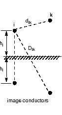
The self and mutual resistance terms are:

Rii=Rint+ΔRiiΩ/km

Rik=ΔRikΩ/km

The self and mutual inductance terms are:

Lii=Lint+μ02πlog2hiri+ΔLiiH/km

Lik=μ02πlogDikdik+ΔLikH/km

The self and mutual potential coefficients terms are:

Pii=12πε0log2hirikm/F

Pik=12πε0logDikdikkm/F

[C]=[P]1F/km

where:

  • µ0 is the permeability of free space = 4π.10−4 H/km

  • ɛ0 is the permittivity of free space = 8.8542.10−9 F/km

  • ri is the radius of conductor i in meters

  • dik is the distance between conductors i and k, in meters

  • Dik is the distance between conductor i and image of k, in meters

  • hi is the average height of conductor i above ground, in meters

  • Rint, Lint are the internal resistance and inductance of conductor

  • ΔRii, ΔRik are the Carson R correction terms due to ground resistivity

  • ΔLii, ΔLik are the Carson L correction terms due to ground resistivity

The conductor self-inductance is computed from the magnetic flux circulating inside and outside the conductor, and produced by the current flowing in the conductor itself. The part of flux circulating inside the conducting material contributes to the internal inductance Lint, which is dependent on the conductor geometry. Assuming a hollow or solid conductor, the internal inductance is computed from the T/D ratio, where D is the conductor diameter and T is the thickness of the conducting material. See the figure Configuration of a Three-Phase Double-Circuit Line. The conductor self-inductance is computed by means of modified Bessel functions from the conductor diameter, T/D ratio, resistivity, and relative permeability of conducting material and specified frequency [1].

The conductor self-inductance can also be computed from parameters that are usually found in tables provided by conductor manufacturers: the Geometric Mean Radius (GMR) or the "Reactance at one-foot spacing."

The GMR is the radius of the equivalent hollow conductor with zero thickness, producing no internal flux, giving the same self-inductance. The conductor self-inductance is then derived from the GMR using the following equation:

Lii=μ02πlog2hiGMR+ΔLiiH/km

For a solid conductor (T/D=0.5), the GMR is

GMR=reμr/4

r = radius of conductor
μr = relative permeability of conducting material

The GMR obtained from this equation assumes a uniform current density in the conductor. This assumption is strictly valid in DC. In AC, the GMR is slightly higher. For example, for a 3 cm diameter solid aluminum conductor (Rdc = 0.040 Ω/km), the GMR increases from 1.1682 cm in DC to 1.1784 cm at 60 Hz. Manufacturers usually give the GMR at the system nominal frequency (50 Hz or 60 Hz).

The reactance Xa at 1-foot spacing (or 1-meter spacing, if metric units are used) is the positive-sequence reactance of a three-phase line having one foot (or one meter) spacing between the three phases and infinite conductor heights. The reactance at 1-foot spacing (or 1-meter spacing) at frequency f is related to the GMR by the following equation:

Xa=ωμ02πlog1GMRΩ/km

GMR = Geometric Mean Radius in feet or meters
ω = 2π.f in rad/s
f = frequency in hertz

The conductor resistance matrix at a particular frequency depends on the DC resistance of the conductor corrected for skin effect and ground resistivity. Both the resistance matrix and the inductance matrix are dependent on the ground resistivity and frequency. Correction terms for the R and L terms as developed by J.R. Carson in 1926 [2] are implemented in power_lineparam.

References

[1] Dommel, H., et al., Electromagnetic Transients Program Reference Manual (EMTP Theory Book), 1986.

[2] Carson, J. R., "Wave Propagation in Overhead Wires with Ground Return," Bell Systems Technical Journal, Vol. 5, pp 539-554, 1926.

Go to top of page