spectralKurtosis

Spectral kurtosis for signals and spectrograms

Syntax

kurtosis = spectralKurtosis(x,f)

kurtosis = spectralKurtosis(xt)

kurtosis = spectralKurtosis(x,f,Name=Value)

[kurtosis,spread,centroid] = spectralKurtosis(___)

[kurtosis,spread,centroid,threshold] = spectralKurtosis(___,ConfidenceLevel=p)

[kurtosis,spread,centroid,threshold,fout] = spectralKurtosis(___)

spectralKurtosis(___)

Description

kurtosis = spectralKurtosis(x,f) returns the spectral kurtosis over time of the time-domain or frequency-domain signal x. How the function interprets x depends on the shape of f.

kurtosis = spectralKurtosis(xt) returns the spectral kurtosis over time of the signal stored in the MATLAB^® timetable xt.

kurtosis = spectralKurtosis(x,f,Name=Value) specifies additional options using one or more name-value arguments. For example, you can specify the window applied for a time-domain input, the amount of overlap between adjacent windows, and the kind of spectrum used for frequency-domain input.

[kurtosis,spread,centroid] = spectralKurtosis(___) returns the spectral spread and spectral centroid. You can specify an input combination from any of the previous syntaxes.

[kurtosis,spread,centroid,threshold] = spectralKurtosis(___,ConfidenceLevel=p) additionally returns the spectral kurtosis threshold using the confidence level p. Kurtosis values beyond threshold indicate regions where the signal has a probability 1 – p of being a stationary Gaussian process. (since R2024b)

[kurtosis,spread,centroid,threshold,fout] = spectralKurtosis(___) additionally returns the frequency values at which the spectral kurtosis is computed. (since R2025a)

spectralKurtosis(___) with no output arguments plots the spectral kurtosis.

• If the input is in the time domain, the spectral kurtosis is plotted against time.

• If the input is in the frequency domain, the spectral kurtosis is plotted against frame number.

Examples

Spectral Kurtosis of Time-Domain Signal

Generate a train of damped sinusoids. The pulses occur every 2 seconds and have exponentially decreasing amplitudes. The signal is sampled at 1 kHz for 10 seconds and is embedded in white Gaussian noise such that the signal-to-noise ratio is 2 dB. Plot the signal.

fs = 1000;
t = (0:1/fs:10-1/fs)';

fnx = @(x,fn) sin(2*pi*fn*x).*exp(-fn*abs(x));

d = 1:2:10;
dd = [d;1.3.^-d]';

SNR = 2;

y = pulstran(t,dd,fnx,10);
y = y + randn(size(t))*std(y)/db2mag(SNR);

plot(t,y)
xlabel("Time (s)")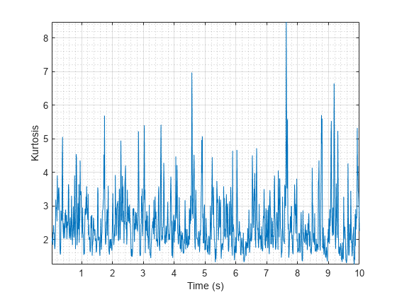

Compute the spectral kurtosis of the signal using default parameters. Plot the spectral kurtosis as a function of time.

krt = spectralKurtosis(y,fs);
plot(linspace(0,t(end),length(krt)),krt)
xlabel("Time (s)")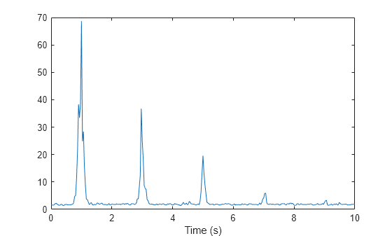

Spectral Kurtosis of Frequency-Domain Signal

Generate a train of damped sinusoids. The pulses occur every 2 seconds and have exponentially decreasing amplitudes. The signal is sampled at 1 kHz for 10 seconds and is embedded in white Gaussian noise such that the signal-to-noise ratio is 2 dB. Use the stft function to compute the spectrogram of the signal.

fs = 1000;
t = (0:1/fs:10-1/fs)';

fnx = @(x,fn) sin(2*pi*fn*x).*exp(-fn*abs(x));

d = 1:2:10;
dd = [d;1.3.^-d]';
SNR = 2;

y = pulstran(t,dd,fnx,10);
x = y+randn(size(t))*std(y)/db2mag(SNR);

[s,f] = stft(x,fs,FrequencyRange="onesided");
s = abs(s).^2;

Compute the kurtosis of the spectrogram over time.

kurtosis = spectralKurtosis(s,f);

Plot the spectral kurtosis as a function of the frame number.

spectralKurtosis(s,f)

Specify Nondefault Parameters

Generate a train of damped sinusoids. The pulses occur every 2 seconds and have exponentially decreasing amplitudes. The signal is sampled at 1 kHz for 10 seconds and is embedded in white Gaussian noise such that the signal-to-noise ratio is 20 dB. Store the signal as a MATLAB timetable.

fs = 1000;
t = (0:1/fs:10-1/fs)';

fnx = @(x,fn) sin(2*pi*fn*x).*exp(-fn*abs(x));

d = 1:2:10;
dd = [d;1.3.^-d]';

SNR = 20;

y = pulstran(t,dd,fnx,12);
rng default
y = y+randn(size(t))*std(y)/db2mag(SNR);

xt = timetable(y,SampleRate=fs);

Calculate the spectral kurtosis over time. Calculate the kurtosis for 50 ms Hamming windows of data with 25 ms overlap. Use the range from 10 Hz to 62.5 Hz for the kurtosis calculation.

kurtosis = spectralKurtosis(xt, ...
    Window=hamming(round(0.05*fs)), ...
    OverlapLength=round(0.025*fs), ...
    Range=[10 62.5]);

Plot the kurtosis as a function of time.

plot(linspace(t(1),t(end),length(kurtosis)),kurtosis)
xlabel("Time (s)")

Spectral Kurtosis of Nonstationary Signal with Different Confidence Levels

Plot the spectral kurtosis of a chirp signal in white noise, and see how the nonstationary non-Gaussian regime can be detected. Explore the effects of changing the confidence level.

Create a chirp signal, add white Gaussian noise, and plot the signal.

fs = 1000;
t = 0:1/fs:10;
f1 = 300;
f2 = 400;

xc = chirp(t,f1,10,f2);
x = xc + randn(1,length(t));

plot(t,x)
title('Chirp Signal with White Gaussian Noise')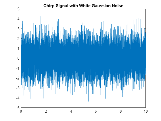

Compute and plot the spectral kurtosis of the signal.

[S,F] = pspectrum(x,fs,"spectrogram", ...
    FrequencyResolution=fs/winlen(length(x)),OverlapPercent=80);

[sK95,~,~,thresh95,fout] = spectralKurtosis(S,F,Scaled=false);

plot(fout,sK95)
yline(thresh95*[-1 1])
grid
xlabel("Frequency (Hz)")
title(["Spectral Kurtosis of Chirp Signal" "in White Gaussian Noise"])

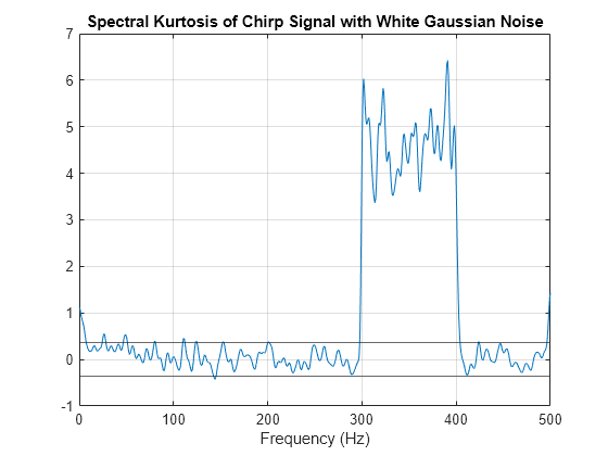
The plot shows a clear extended excursion from 300 Hz to 400 Hz. This excursion corresponds to the signal component that represents the nonstationary chirp. The area between the two horizontal lines represents the zone of probable stationary and Gaussian behavior, as defined by the 0.95 confidence interval. Any kurtosis points falling within this zone are likely to be stationary and Gaussian. Outside of the zone, kurtosis points are flagged as nonstationary or non-Gaussian. Below 300 Hz, there are a few additional excursions slightly above the zone threshold. These excursions represent false positives, where the signal is stationary and Gaussian, but because of the noise, has exceeded the threshold.

Investigate the impact of the confidence level by changing it from the default 0.95 to 0.75.

cl = 0.75;

[sK75,~,~,thresh75] = spectralKurtosis(S,F,Scaled=false,ConfidenceLevel=cl);

plot(fout,sK75)
yline(thresh75*[-1 1])
grid
xlabel("Frequency (Hz)")
title(["Spectral Kurtosis of Chirp Signal" "in Noise at Confidence Level "+cl])

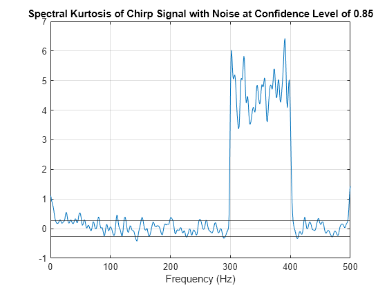
The lower confidence level implies more sensitive detection of nonstationary or non-Gaussian frequency components. Reducing the confidence level shrinks the threshold-delimited zone. Now the low-level excursions—false alarms—have increased in both number and amount. Setting the confidence level is a balancing act between achieving effective detection and limiting the number of false positives.

Compare the zone width for the two cases.

thresh = [thresh95 thresh75]

thresh = 1×2

    0.3578    0.2100

function y = winlen(x)
    wdiv = 2.^[1 3:7];
    y = ceil(x/wdiv(find(x < 2.^[6 11:14 Inf],1)));
end

Input Arguments

x — Input signal

column vector | matrix | 3-D array

Input signal, specified as a column vector, a matrix, or a 3-D array. How the function interprets x depends on the shape of f.

Data Types: single | double

xt — Input timetable

timetable

Since R2024b

Input timetable. spectralKurtosis infers the sample rate from xt.

Example: timetable(randn(5000,1),SampleRate=1e3) specifies a random variable sampled at 1 kHz for 5 seconds.

Data Types: single | double

f — Sample rate, sample time, or frequency vector

numeric scalar | duration scalar | vector

Sample rate, sample time, or frequency vector in Hz, specified as a numeric scalar, a duration scalar, or a vector. How the function interprets x depends on the shape of f:

• If f is not specified and x is a numeric vector or matrix, spectralKurtosis assumes x is sampled at a rate equal to 1 Hz.

• If f is a numeric scalar, spectralKurtosis interprets x as a time-domain signal and f as a sample rate. In this case, x must be a real vector or matrix. If x is a matrix, spectralKurtosis interprets its columns as individual channels.

• If f is a duration scalar, spectralKurtosis interprets x as a time-domain signal and f as a sample time (since R2025a). In this case, x must be a real vector or matrix. If x is a matrix, spectralKurtosis interprets its columns as individual channels.

• If f is a vector, spectralKurtosis interprets x as a frequency-domain signal and f as the frequencies, in Hz, corresponding to the rows of x. In this case, x must be a real L-by-M-by-N array, where L is the number of spectral values at given frequencies of f, M is the number of individual spectra, and N is the number of channels.

  The number of rows of x must equal the number of elements of f.

Data Types: single | double | duration (since R2025a)

Name-Value Arguments

Specify optional pairs of arguments as Name1=Value1,...,NameN=ValueN, where Name is the argument name and Value is the corresponding value. Name-value arguments must appear after other arguments, but the order of the pairs does not matter.

Before R2021a, use commas to separate each name and value, and enclose Name in quotes.

Example: Window=hamming(256),OverlapLength=128 divides a time-domain input signal into 256-sample segments, specifies 128 samples of overlap between adjoining segments, and windows each segment with a Hamming window.

Note

The following name-value arguments apply if x is a time-domain signal. If x is a frequency-domain signal, only the Scaled and ConfidenceLevel arguments apply.

Window — Window applied in time domain

rectwin(round(f*0.03)) (default) | vector

Window applied in the time domain, specified as a real vector. The number of elements in the vector must be in the range [1, size(x,1)]. The number of elements in the vector must also be greater than OverlapLength. If you do not specify Window, spectralKurtosis uses a window length that splits x into eight overlapping segments.

Data Types: single | double

OverlapLength — Number of samples overlapped between adjacent windows

round(f*0.02) (default) | nonnegative scalar integer

Number of samples overlapped between adjacent windows, specified as an integer in the range [0, size(Window,1)). If you do not specify OverlapLength, spectralKurtosis uses a value that results in 50% overlap between segments.

Data Types: single | double

FFTLength — Number of bins in DFT

numel(Window) (default) | positive scalar integer

Number of bins used to calculate the DFT of windowed input samples, specified as a positive scalar integer. If unspecified, FFTLength defaults to the number of elements in the Window.

Data Types: single | double

Range — Frequency range (Hz)

[0,f/2] (default) | two-element row vector

Frequency range in Hz, specified as a two-element row vector of increasing real values in the range [0, f/2].

Data Types: single | double

SpectrumType — Spectrum type

"power" (default) | "magnitude"

Spectrum type, specified as "power" or "magnitude".

• "power" –– The function calculates spectral kurtosis for the one-sided power spectrum.

• "magnitude" –– The function calculates spectral kurtosis for the one-sided magnitude spectrum.

Data Types: char | string

Scaled — Scale option

true (default) | false

Since R2024b

Scale option, specified as a logical true or false. This argument specifies how the function computes spectral kurtosis. If Scaled is true, spectralKurtosis returns the frequency-averaged spectral kurtosis. If Scaled is false, spectralKurtosis returns the numeric kurtosis of the signal spectrogram.

This argument applies if x is a time- or frequency-domain signal.

Data Types: logical

ConfidenceLevel — Confidence level

0.95 (default) | [0 to 1]

Since R2024b

Confidence level used to determine whether the input signal is likely to be Gaussian and stationary, specified as a numeric scalar value from 0 to 1. This argument influences the threshold range where the spectral kurtosis value indicates a Gaussian and stationary signal. The confidence level therefore provides a detection-sensitivity tuning parameter. Kurtosis values outside of this range indicate non-Gaussian or nonstationary behavior.

This argument applies only if Scaled is false.

Data Types: single | double

Output Arguments

kurtosis — Spectral kurtosis

scalar | vector | matrix

Spectral kurtosis, returned as a scalar, vector, or matrix. Each row of kurtosis corresponds to the spectral kurtosis of a window of x. Each column of kurtosis corresponds to an independent channel.

spread — Spectral spread

scalar | vector | matrix

Spectral spread, returned as a scalar, vector, or matrix. Each row of spread corresponds to the spectral spread of a window of x. Each column of spread corresponds to an independent channel.

centroid — Spectral centroid

scalar | vector | matrix

Spectral centroid in Hz, returned as a scalar, vector, or matrix. Each row of centroid corresponds to the spectral centroid of a window of x. Each column of centroid corresponds to an independent channel.

threshold — Spectral kurtosis band size for stationary Gaussian behavior

scalar

Since R2024b

Spectral kurtosis band size for stationary Gaussian behavior, returned as a numeric scalar. Signal regions with kurtosis values larger than threshold exhibit nonstationarity or non-Gaussianity with a confidence p specified using ConfidenceLevel. In other words, wherever the kurtosis is beyond the threshold, the signal has a probability 1 – p of being a stationary Gaussian process.

If Scaled is true, spectralKurtosis returns an empty vector as fourth output.

fout — Frequency vector

vector

Since R2025a

Frequencies associated with kurtosis values, returned as a vector in hertz.

More About

Spectral Kurtosis

Spectral kurtosis (SK) is a statistical tool that can indicate and pinpoint nonstationary or non-Gaussian behavior in the frequency domain, by taking:

• Small values at frequencies where only stationary Gaussian noise is present

• High positive values at frequencies where transients occur

This capability makes SK a powerful tool for detecting and extracting signals associated with faults in rotating mechanical systems. On its own, SK can identify features or conditional indicators for fault detection and classification. As preprocessing for other tools such as envelope analysis, SK can supply key inputs such as optimal band [1], [2].

The spectral kurtosis, or K(f), of a signal x(t) can be computed based on the short-time Fourier transform (STFT) of the signal, S(t,f):

$$S\left(t,f\right)={\displaystyle {\int }_{-\infty }^{\infty }x\left(\tau \right)w\left(\tau -t\right)e^{-j2\pi f\tau }d\tau },$$

where w(t) is the window function used in the STFT.

• If you specify Scaled as true, spectralKurtosis computes the spectral kurtosis as described in [3]:

  $$\text{kurtosis}=\frac{{\displaystyle \sum _{k=b_1}^{b_2}{\left(f_k-{\mu }_1\right)}^4{s}_k}}{{\left({\mu }_2\right)}^4{\displaystyle \sum _{k=b_1}^{b_2}{s}_k}},$$

  where:

  • f_k is the frequency in Hz corresponding to bin k.

  • s_k is the spectral value at bin k.

  • b₁ and b₂ are the band edges, in bins, over which to calculate the spectral kurtosis.

  • μ₁ is the spectral centroid, calculated as described by the spectralCentroid (Audio Toolbox) function.

  • μ₂ is the spectral spread, calculated as described by the spectralSpread (Audio Toolbox) function.

• If you specify Scaled as false, spectralKurtosis computes the spectral kurtosis K(f) as

  $$K(f)=\frac{{\langle {\left|S(t,f)\right|}^4\rangle }_t}{{\langle {\left|S(t,f)\right|}^2\rangle }_t^2}-2,f\ne 0,$$

  where 〈·〉_t is the time-average operator.

  If the signal x(t) contains only stationary Gaussian noise, then K(f) at each frequency f has an asymptotic normal distribution with 0 mean and variance 4/M, where M is the number of elements along the time axis in S(t,f). Hence, a statistical threshold s_α given a confidence level α is

  $$s_{\alpha }={\Phi }^{-1}\left(\alpha \right)\frac{2}{\sqrt{M}},$$

  where $${\Phi }^{-1}(\alpha )=\sqrt{2}{\mathrm{erf}}^{-1}(2\alpha -1)$$ is the quantile function of the standard normal distribution.

  It is important to note that the STFT window length N_w directly drives frequency resolution, which is f_s/N_w, where f_s is the sample rate. The window size must be shorter than the spacing between transient impulses but longer than the individual transient impulses.

References

[1] Antoni, J. "The Spectral Kurtosis: A Useful Tool for Characterising Non-Stationary Signals." Mechanical Systems and Signal Processing. Vol. 20, Issue 2, 2006, pp. 282–307.

[2] Antoni, J., and R. B. Randall. "The Spectral Kurtosis: Application to the Vibratory Surveillance and Diagnostics of Rotating Machines." Mechanical Systems and Signal Processing. Vol. 20, Issue 2, 2006, pp. 308–331.

[3] Peeters, G. "A Large Set of Audio Features for Sound Description (Similarity and Classification) in the CUIDADO Project." Technical Report; IRCAM: Paris, France, 2004.

Extended Capabilities

C/C++ Code Generation
Generate C and C++ code using MATLAB® Coder™.

GPU Arrays
Accelerate code by running on a graphics processing unit (GPU) using Parallel Computing Toolbox™.

Version History

Introduced in R2019a

R2025a: Specify sample time and return frequency vector

The spectralKurtosis function supports specifying a sample time for the input signal as a duration scalar. You can also obtain the vector of frequencies at which the spectral kurtosis is computed.

R2024b: Use timetable input and customize feature extraction

The spectralKurtosis function supports MATLAB timetables as input. You can set the Scaled argument to false to obtain the numeric kurtosis of the spectrogram of the input signal. You can use the ConfidenceLevel argument to specify the width of the range within which an input signal is determined to be Gaussian and stationary.

R2024b: Recommended over pkurtosis

The pkurtosis function will be removed in a future release. Use spectralKurtosis instead.