findchangepts

Find abrupt changes in signal

Syntax

ipt = findchangepts(x)

ipt = findchangepts(x,Name,Value)

[ipt,residual] = findchangepts(___)

findchangepts(___)

Description

ipt = findchangepts(x) returns the index at which the mean of x changes most significantly.

• If x is a vector with N elements, then findchangepts partitions x into two regions, x(1:ipt-1) and x(ipt:N), that minimize the sum of the residual (squared) error of each region from its local mean.

• If x is an M-by-N matrix, then findchangepts partitions x into two regions, x(1:M,1:ipt-1) and x(1:M,ipt:N), returning the column index that minimizes the sum of the residual error of each region from its local M-dimensional mean.

ipt = findchangepts(x,Name,Value) specifies additional options using name-value arguments. Options include the number of changepoints to report and the statistic to measure instead of the mean. See Changepoint Detection for more information.

[ipt,residual] = findchangepts(___) also returns the residual error of the signal against the modeled changes, incorporating any of the previous specifications.

findchangepts(___) without output arguments plots the signal and any detected changepoints. For more information, see Statistic.

Note

Before plotting, the findchangepts function clears (clf) the current figure. To plot the signal and detected changepoints in a subplot, use a plotting function. See Audio File Segmentation.

Examples

Changepoints in One and Two Dimensions

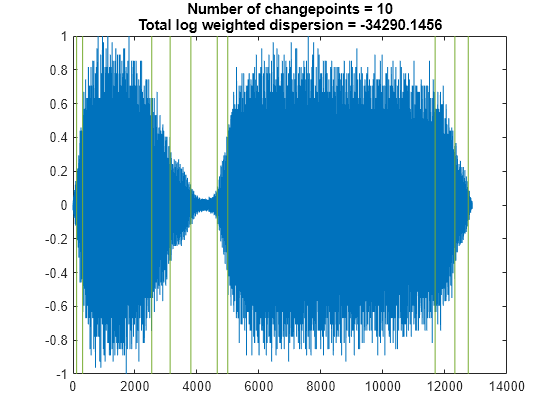
Load a data file containing a recording of a train whistle sampled at 8192 Hz. Find the 10 points at which the root-mean-square level of the signal changes most significantly.

load train

findchangepts(y,MaxNumChanges=10,Statistic="rms")

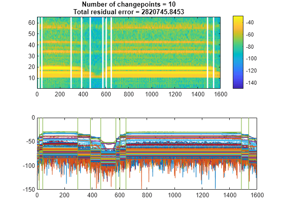
Compute the short-time power spectral density of the signal. Divide the signal into 128-sample segments and window each segment with a Hamming window. Specify 120 samples of overlap between adjoining segments and 128 DFT points. Find the 10 points at which the mean of the power spectral density changes the most significantly.

[s,f,t,pxx] = spectrogram(y,128,120,128,Fs);

findchangepts(pow2db(pxx),MaxNumChanges=10)

Changepoint Search Options

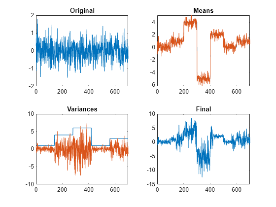
Reset the random number generator for reproducible results. Generate a random signal where:

• The mean is constant in each of seven regions and changes abruptly from region to region.

• The variance is constant in each of five regions and changes abruptly from region to region.

rng("default")

lr = 20;

mns = [0 1 4 -5 2 0 1];
nm = length(mns);

vrs = [1 4 6 1 3];
nv = length(vrs);

v = randn(1,lr*nm*nv)/2;

f = reshape(repmat(mns,lr*nv,1),1,lr*nm*nv);
y = reshape(repmat(vrs,lr*nm,1),1,lr*nm*nv);

t = v.*y+f;

Plot the signal, highlighting the steps of its construction.

subplot(2,2,1)
plot(v)
title("Original")
xlim([0 700])

subplot(2,2,2)
plot([f;v+f]')
title("Means")
xlim([0 700])

subplot(2,2,3)
plot([y;v.*y]')
title("Variances")
xlim([0 700])

subplot(2,2,4)
plot(t)
title("Final")
xlim([0 700])

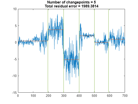
Find the five points where the mean of the signal changes most significantly.

figure
findchangepts(t,MaxNumChanges=5)

Find the five points where the root-mean-square level of the signal changes most significantly.

findchangepts(t,MaxNumChanges=5,Statistic="rms")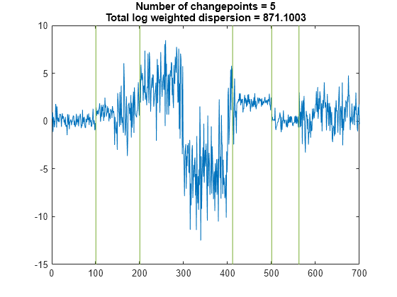

Find the point where the mean and standard deviation of the signal change the most.

findchangepts(t,Statistic="std")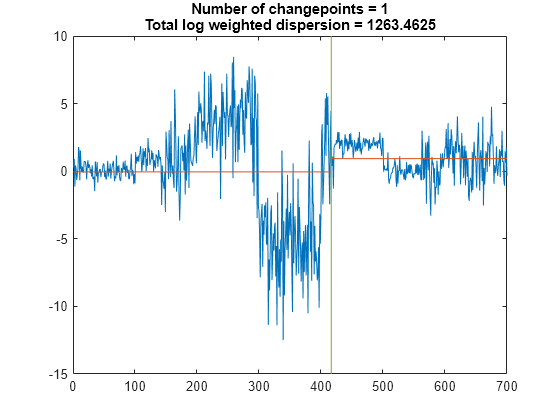

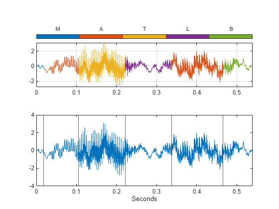
Audio File Segmentation

Load a speech signal sampled at $$F_s=7418Hz$$. The file contains a recording of a female voice saying the word "MATLAB®."

load mtlb

Discern the vowels and consonants in the word by finding the points at which the variance of the signal changes significantly. Limit the number of changepoints to five.

numc = 5;

[q,r] = findchangepts(mtlb,Statistic="rms",MaxNumChanges=numc);

Create a signal mask for the speech signal based on the changepoint indices. See signalMask for more information about using a signal mask.

t = (0:length(mtlb)-1)/Fs;
roitable = ([[1;q] [q;length(mtlb)]]);

x = ["M" "A" "T" "L" "A" "B"]';
c = categorical(x,unique(x,"stable"));

msk = signalMask(table(t(roitable),c),SampleRate=Fs,RightShortening=1);
roimask(msk)

ans=6×2 table
           Var1            c
    ___________________    _

          0    0.017525    M
    0.01766     0.10461    A
    0.10475     0.22162    T
    0.22176     0.33675    L
    0.33688     0.46535    A
    0.46549     0.53909    B

Plot the speech signal and detected changepoints in a subplot along with the regions of interest from the signal mask:

• In the upper subplot, use the plotsigroi function to visualize the signal mask regions. Adjust the settings to make the colorbar appear at the top..

• In the lower subplot, plot the original speech signal and add the detected changepoints as vertical lines.

subplot(2,1,1)
plotsigroi(msk,mtlb)
colorbar("off")
nc = numel(c)-1;
colormap(gca,lines(nc));
colorbar(TickLabels=categories(c),Ticks=1/2/nc:1/nc:1, ...
    TickLength=0,Location="northoutside")
xlabel("")

subplot(2,1,2)
plot(t,mtlb)
hold on
xline(q/Fs)
hold off
xlim([0 t(end)])
xlabel("Seconds")

To play the sound with a pause after each of the segments, uncomment these lines.

% for k = 1:length(roitable)
%     intv = roitable(k,1):roitable(k,2);
%     soundsc(mtlb(intv).*hann(length(intv)),Fs)
%     pause(.5)
% end

Change of Mean, RMS Level, Standard Deviation, and Slope

Create a signal that consists of two sinusoids with varying amplitude and a linear trend.

vc = sin(2*pi*(0:201)/17).*sin(2*pi*(0:201)/19).* ...
    [sqrt(0:0.01:1) (1:-0.01:0).^2]+(0:201)/401;

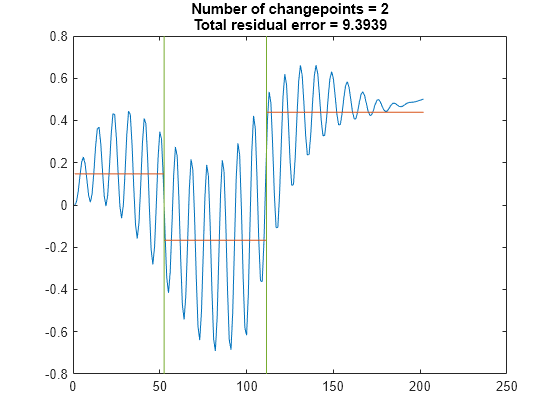
Find the points where the signal mean changes most significantly. The 'Statistic' name-value argument is optional in this case. Specify a minimum residual error improvement of 1.

findchangepts(vc,'Statistic','mean','MinThreshold',1)

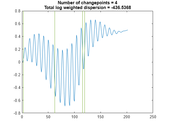
Find the points where the root-mean-square level of the signal changes the most. Specify a minimum residual error improvement of 6.

findchangepts(vc,'Statistic','rms','MinThreshold',6)

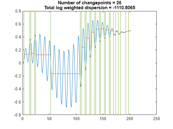
Find the points where the standard deviation of the signal changes most significantly. Specify a minimum residual error improvement of 10.

findchangepts(vc,'Statistic','std','MinThreshold',10)

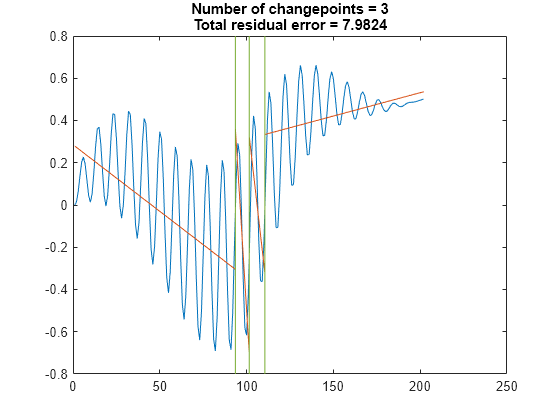
Find the points where the mean and the slope of the signal change most abruptly. Specify a minimum residual error improvement of 0.6.

findchangepts(vc,'Statistic','linear','MinThreshold',0.6)

Changepoints of 2-D and 3-D Bézier Curves

Generate a two-dimensional, 1000-sample Bézier curve with 20 random control points. A Bézier curve is defined by:

$$C(t)={\displaystyle \sum _{k=0}^m\left(\genfrac{}{}{0ex}{}{m}{k}\right)t^k(1-t{)}^{m-k}{P}_k}$$,

where ${\mathit{P}}_{\mathit{k}}$ is the $\mathit{k}$th of $\mathit{m}$ control points, $\mathit{t}$ ranges from 0 to 1, and $$\left(\genfrac{}{}{0ex}{}{m}{k}\right)$$ is a binomial coefficient. Plot the curve and the control points.

m = 20;
P = randn(m,2);
t = linspace(0,1,1000)';

pol = t.^(0:m-1).*(1-t).^(m-1:-1:0);
bin = gamma(m)./gamma(1:m)./gamma(m:-1:1);
crv = bin.*pol*P;

plot(crv(:,1),crv(:,2),P(:,1),P(:,2),"o:")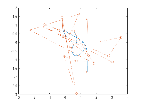

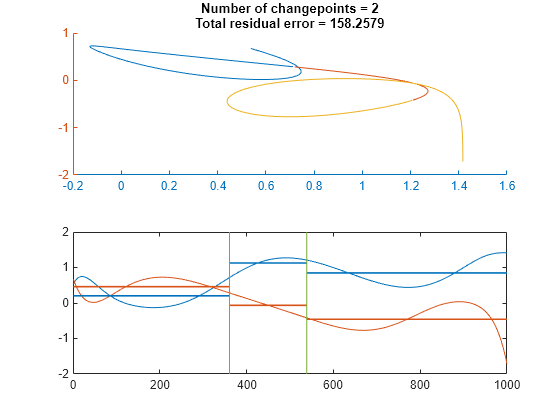
Partition the curve into three segments, such that the points in each segment are at a minimum distance from the segment mean.

findchangepts(crv',MaxNumChanges=3)

Partition the curve into 20 segments that are best fit by straight lines.

findchangepts(crv',Statistic="linear",MaxNumChanges=19)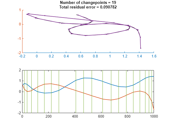

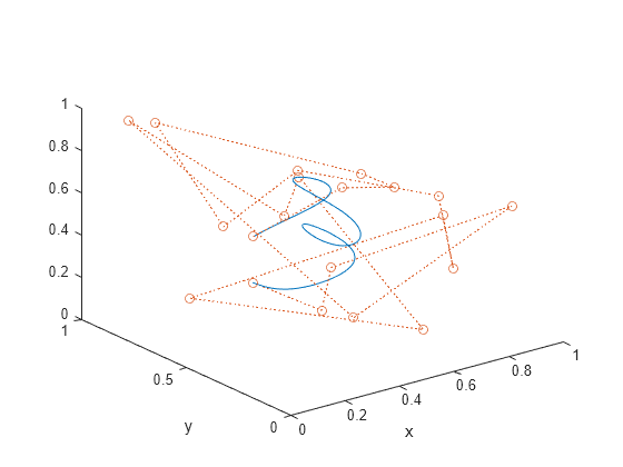
Generate and plot a three-dimensional Bézier curve with 20 random control points.

P = rand(m,3);
crv = bin.*pol*P;

plot3(crv(:,1),crv(:,2),crv(:,3),P(:,1),P(:,2),P(:,3),"o:")
xlabel("x")
ylabel("y")

Visualize the curve from above.

view([0 0 1])

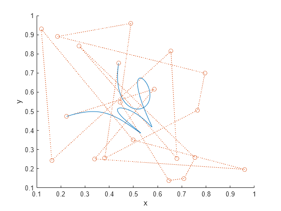
Partition the curve into three segments, such that the points in each segment are at a minimum distance from the segment mean.

findchangepts(crv',MaxNumChanges=3)

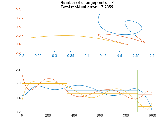
Partition the curve into 20 segments that are best fit by straight lines.

findchangepts(crv',Statistic="linear",MaxNumChanges=19)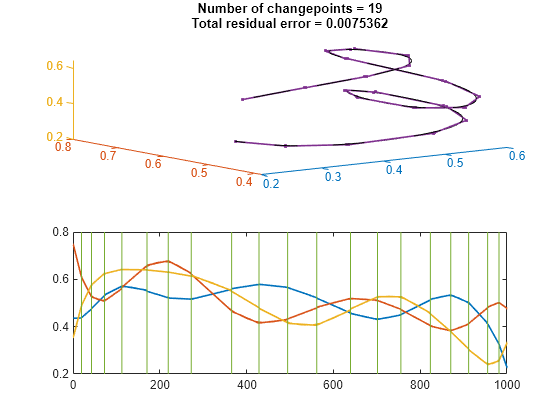

Input Arguments

x — Input signal

real-valued vector | real-valued matrix

Input signal, specified as a real-valued vector or matrix.

• If x is a vector with N elements, then findchangepts partitions x into two regions, x(1:ipt-1) and x(ipt:N), that minimize the sum of the residual (squared) error of each region from the local value of the statistic specified in Statistic.

• If x is an M-by-N matrix, then findchangepts partitions x into two regions, x(1:M,1:ipt-1) and x(1:M,ipt:N), returning the column index that minimizes the sum of the residual error of each region from the local M-dimensional value of the statistic specified in Statistic.

Example: reshape(randn(100,3)+[-3 0 3],1,300) is a random signal with two abrupt changes in mean.

Example: reshape(randn(100,3).*[1 20 5],1,300) is a random signal with two abrupt changes in root-mean-square level.

Data Types: single | double

Name-Value Arguments

Specify optional pairs of arguments as Name1=Value1,...,NameN=ValueN, where Name is the argument name and Value is the corresponding value. Name-value arguments must appear after other arguments, but the order of the pairs does not matter.

Example: MaxNumChanges=3,Statistic="rms",MinDistance=20 finds up to three points where the changes in root-mean-square level are most significant and where the points are separated by at least 20 samples.

Before R2021a, use commas to separate each name and value, and enclose Name in quotes.

Example: 'MaxNumChanges',3,'Statistic',"rms",'MinDistance',20 finds up to three points where the changes in root-mean-square level are most significant and where the points are separated by at least 20 samples.

MaxNumChanges — Maximum number of significant changes to return

1 (default) | integer scalar

Maximum number of significant changes to return, specified as an integer scalar. After finding the point with the most significant change, findchangepts gradually loosens its search criterion to include more changepoints without exceeding the specified maximum. If any search setting returns more than the maximum, then the function returns nothing. If MaxNumChanges is not specified, then the function returns the point with the most significant change. You cannot specify MinThreshold and MaxNumChanges simultaneously.

Example: findchangepts([0 1 0]) returns the index of the second sample.

Example: findchangepts([0 1 0],MaxNumChanges=1) returns an empty matrix.

Example: findchangepts([0 1 0],MaxNumChanges=2) returns the indices of the second and third points.

Data Types: single | double

Statistic — Type of change to detect

"mean" (default) | "rms" | "std" | "linear"

Type of change to detect, specified as one of these values:

• "mean" — Detect changes in mean. If you call findchangepts with no output arguments, the function plots the signal, the changepoints, and the mean value of each segment enclosed by consecutive changepoints.

• "rms" — Detect changes in root-mean-square level. If you call findchangepts with no output arguments, the function plots the signal and the changepoints.

• "std" — Detect changes in standard deviation, using Gaussian log-likelihood. If you call findchangepts with no output arguments, the function plots the signal, the changepoints, and the mean value of each segment enclosed by consecutive changepoints.

• "linear" — Detect changes in mean and slope. If you call findchangepts with no output arguments, the function plots the signal, the changepoints, and the line that best fits each portion of the signal enclosed by consecutive changepoints.

Example: findchangepts([0 1 2 1],Statistic="mean") returns the index of the second sample.

Example: findchangepts([0 1 2 1],Statistic="rms") returns the index of the third sample.

MinDistance — Minimum number of samples between changepoints

integer scalar

Minimum number of samples between changepoints, specified as an integer scalar. If you do not specify this number, then the default is 1 for changes in mean and 2 for other changes.

Example: findchangepts(sin(2*pi*(0:10)/5),MaxNumChanges=5,MinDistance=1) returns five indices.

Example: findchangepts(sin(2*pi*(0:10)/5),MaxNumChanges=5,MinDistance=3) returns two indices.

Example: findchangepts(sin(2*pi*(0:10)/5),MaxNumChanges=5,MinDistance=5) returns no indices.

Data Types: single | double

MinThreshold — Minimum improvement in total residual error

real scalar

Minimum improvement in total residual error for each changepoint, specified as a real scalar that represents a penalty. This option acts to limit the number of returned significant changes by applying the additional penalty to each prospective changepoint. You cannot specify MinThreshold and MaxNumChanges simultaneously.

Example: findchangepts([0 1 2],MinThreshold=0) returns two indices.

Example: findchangepts([0 1 2],MinThreshold=1) returns one index.

Example: findchangepts([0 1 2],MinThreshold=2) returns no indices.

Data Types: single | double

Output Arguments

ipt — Changepoint locations

vector

Changepoint locations, returned as a vector of integer indices.

residual — Residual error

vector

Residual error of the signal against the modeled changes, returned as a vector.

More About

Changepoint Detection

A changepoint is a sample or time instant at which some statistical property of a signal changes abruptly. The property in question can be the mean of the signal, its variance, or a spectral characteristic, among others.

To find a signal changepoint, findchangepts employs a parametric global method. The function:

1. Chooses a point and divides the signal into two sections.

2. Computes an empirical estimate of the desired statistical property for each section.

3. At each point within a section, measures how much the property deviates from the empirical estimate. Adds the deviations for all points.

4. Adds the deviations section-to-section to find the total residual error.

5. Varies the location of the division point until the total residual error attains a minimum.

The procedure is clearest when the chosen statistic is the mean. In that case, findchangepts minimizes the total residual error from the "best" horizontal level for each section. Given a signal x₁, x₂, …, x_N, and the subsequence mean and variance

$$\begin{array}{c}\mathrm{mean}\left(\left[\begin{array}{ccc}{x}_m& \cdots & x_n\end{array}\right]\right)=\frac{1}{n-m+1}{\displaystyle \sum _{r=m}^n{x}_r,}\\ \mathrm{var}\left(\left[\begin{array}{ccc}{x}_m& \cdots & x_n\end{array}\right]\right)=\frac{1}{n-m+1}{\displaystyle \sum _{r=m}^n{\left(x_r-\mathrm{mean}\left(\left[\begin{array}{ccc}{x}_m& \cdots & x_n\end{array}\right]\right)\right)}^2\equiv \frac{{S_{xx}|}_m^n}{n-m+1}},\end{array}$$

where the sum of squares

$${S_{xy}|}_m^n\equiv {\displaystyle \sum _{r=m}^n\left(x_r-\mathrm{mean}\left(\left[\begin{array}{ccc}{x}_m& \cdots & x_n\end{array}\right]\right)\right)\left(y_r-\mathrm{mean}\left(\left[\begin{array}{ccc}{y}_m& \cdots & y_n\end{array}\right]\right)\right)},$$

findchangepts finds k such that the total residual error

$$\begin{array}{c}J={\displaystyle \sum _{i=1}^{k-1}{\left(x_i-\mathrm{mean}\left(\left[\begin{array}{ccc}{x}_1& \cdots & x_{k-1}\end{array}\right]\right)\right)}^2}+{\displaystyle \sum _{i=k}^N{\left(x_i-\mathrm{mean}\left(\left[\begin{array}{ccc}{x}_k& \cdots & x_N\end{array}\right]\right)\right)}^2}\\ =\left(k-1\right)\mathrm{var}\left(\left[\begin{array}{ccc}{x}_1& \cdots & x_{k-1}\end{array}\right]\right)+\left(N-k+1\right)\mathrm{var}\left(\left[\begin{array}{ccc}{x}_k& \cdots & x_N\end{array}\right]\right)\end{array}$$

is smallest. This result can be generalized to incorporate other statistics. findchangepts finds k such that the total residual error

$$J\left(k\right)={\displaystyle \sum _{i=1}^{k-1}\Delta \left(x_i;\chi \left(\left[\begin{array}{ccc}{x}_1& \cdots & x_{k-1}\end{array}\right]\right)\right)}+{\displaystyle \sum _{i=k}^N\Delta \left(x_i;\chi \left(\left[\begin{array}{ccc}{x}_k& \cdots & x_N\end{array}\right]\right)\right)}$$

is smallest, given the section empirical estimate χ and the deviation measurement Δ.

Minimizing the residual error is equivalent to maximizing the log likelihood. Given a normal distribution with mean μ and variance σ², the log-likelihood for N independent observations is

$$\log {\displaystyle \prod _{i=1}^N\frac{1}{\sqrt{2\pi {\sigma }^2}}{e}^{-{\left(x_i-\mu \right)}^2/2{\sigma }^2}}=-\frac{N}{2}\left(\log 2\pi +\log {\sigma }^2\right)-\frac{1}{2{\sigma }^2}{\displaystyle \sum _{i=1}^N{\left(x_i-\mu \right)}^2}.$$

• If Statistic is specified as "mean", the variance is fixed and the function uses

  $$\begin{array}{c}{\displaystyle \sum _{i=m}^n\Delta \left(x_i;\chi \left(\left[\begin{array}{ccc}{x}_m& \cdots & x_n\end{array}\right]\right)|\right)}={\displaystyle \sum _{i=m}^n{\left(x_i-\mathrm{mean}\left(\left[\begin{array}{ccc}{x}_m& \cdots & x_n\end{array}\right]\right)\right)}^2}\\ =(n-m+1)\mathrm{var}\left(\left[\begin{array}{ccc}{x}_m& \cdots & x_n\end{array}\right]\right),\end{array}$$

  as obtained previously.

• If Statistic is specified as "std", the mean is fixed and the function uses

  $$\begin{array}{c}{\displaystyle \sum _{i=m}^n\Delta \left(x_i;\chi \left(\left[\begin{array}{ccc}{x}_m& \cdots & x_n\end{array}\right]\right)\right)}=\left(n-m+1\right)\log {\displaystyle \sum _{i=m}^n{\sigma }^2\left(\left[\begin{array}{ccc}{x}_m& \cdots & x_n\end{array}\right]\right)}\\ =\left(n-m+1\right)\log \left(\frac{1}{n-m+1}{\displaystyle \sum _{i=m}^n{\left(x_i-\mathrm{mean}\left(\left[\begin{array}{ccc}{x}_m& \cdots & x_n\end{array}\right]\right)\right)}^2}\right)\\ =\left(n-m+1\right)\log \mathrm{var}\left(\left[\begin{array}{ccc}{x}_m& \cdots & x_n\end{array}\right]\right).\end{array}$$

• If Statistic is specified as "rms", the total deviation is the same as for "std" but with the mean set to zero:

  $${\displaystyle \sum _{i=m}^n\Delta \left(x_i;\chi \left(\left[\begin{array}{ccc}{x}_m& \cdots & x_n\end{array}\right]\right)\right)}=\left(n-m+1\right)\log \left(\frac{1}{n-m+1}{\displaystyle \sum _{r=m}^n{x}_r^2}\right).$$

• If Statistic is specified as "linear", the function uses as total deviation the sum of squared differences between the signal values and the predictions of the least-squares linear fit through the values. This quantity is also known as the error sum of squares, or SSE. The best-fit line through x_m, x_m+1, …, x_n is

  $$\widehat{x}\left(t\right)=\frac{{S_{xt}|}_m^n}{{S_{tt}|}_m^n}\left(t-\mathrm{mean}\left(\left[\begin{array}{ccc}{t}_m& \cdots & t_n\end{array}\right]\right)\right)+\mathrm{mean}\left(\left[\begin{array}{ccc}{x}_m& \cdots & x_n\end{array}\right]\right)$$

  and the SSE is

  $$\begin{array}{c}{\displaystyle \sum _{i=m}^n\Delta \left(x_i;\chi \left(\left[\begin{array}{ccc}{x}_m& \cdots & x_n\end{array}\right]\right)\right)}={\displaystyle \sum _{i=m}^n{\left(x_i-\widehat{x}\left(t_i\right)\right)}^2}\\ ={S_{xx}|}_m^n-\frac{{S_{xt}^2|}_m^n}{{S_{tt}|}_m^n}\\ =\left(n-m+1\right)\mathrm{var}\left(\left[\begin{array}{ccc}{x}_m& \cdots & x_n\end{array}\right]\right)\\ -\frac{{\left({\displaystyle \sum _{i=m}^n\left(x_i-\mathrm{mean}\left(\left[\begin{array}{ccc}{x}_m& \cdots & x_n\end{array}\right]\right)\right)\left(i-\mathrm{mean}\left(\left[\begin{array}{cccc}m& m+1& \cdots & n\end{array}\right]\right)\right)}\right)}^2}{\left(n-m+1\right)\mathrm{var}\left(\left[\begin{array}{cccc}m& m+1& \cdots & n\end{array}\right]\right)}.\end{array}$$

Signals of interest often have more than one changepoint. Generalizing the procedure is straightforward when the number of changepoints is known. When the number is unknown, you must add a penalty term to the residual error, since adding changepoints always decreases the residual error and results in overfitting. In the extreme case, every point becomes a changepoint and the residual error vanishes. findchangepts uses a penalty term that grows linearly with the number of changepoints. If there are K changepoints to be found, then the function minimizes

$$J\left(K\right)={\displaystyle \sum _{r=0}^{K-1}{\displaystyle \sum _{i=k_r}^{k_{r+1}-1}\Delta \left(x_i;\chi \left(\left[\begin{array}{ccc}{x}_{k_r}& \cdots & x_{k_{r+1}-1}\end{array}\right]\right)\right)}+\beta K,}$$

where k₀ and k_K are respectively the first and the last sample of the signal.

• The proportionality constant, denoted by β and specified in MinThreshold, corresponds to a fixed penalty added for each changepoint. findchangepts rejects adding additional changepoints if the decrease in residual error does not meet the threshold. Set MinThreshold to zero to return all possible changes.

• If you do not know what threshold to use or have a rough idea of the number of changepoints in the signal, specify MaxNumChanges instead. This option gradually increases the threshold until the function finds fewer changes than the specified value.

To perform the minimization itself, findchangepts uses an exhaustive algorithm based on dynamic programming with early abandonment.

References

[1] Killick, Rebecca, Paul Fearnhead, and Idris A. Eckley. “Optimal detection of changepoints with a linear computational cost.” Journal of the American Statistical Association. Vol. 107, No. 500, 2012, pp. 1590–1598.

[2] Lavielle, Marc. “Using penalized contrasts for the change-point problem.” Signal Processing. Vol. 85, August 2005, pp. 1501–1510.

Extended Capabilities

C/C++ Code Generation

Generate C and C++ code using MATLAB® Coder™.

Usage notes and limitations:

• If you specify input argument Statistic, then it must be a compile-time constant.

Version History

Introduced in R2016a