2-D Path Tracing with Inverse Kinematics
Introduction
This example shows how to calculate inverse kinematics for a simple 2-D manipulator using the inverseKinematics class. The manipulator robot is a simple 2-degree-of-freedom planar manipulator with revolute joints which is created by assembling rigid bodies into a rigidBodyTree object. A circular trajectory is created in a 2-D plane and given as points to the inverse kinematics solver. The solver calculates the required joint positions to achieve this trajectory. Finally, the robot is animated to show the robot configurations that achieve the circular trajectory.
Construct the Robot
Create a rigidBodyTree object and rigid bodies with their associated joints. Specify the geometric properties of each rigid body and add it to the robot.
Start with a blank rigid body tree model.
robot = rigidBodyTree('DataFormat','column','MaxNumBodies',3);
Specify arm lengths for the robot arm.
L1 = 0.3;
L2 = 0.3;
Specify the length of the offset for the tool tip along the X-axis of the tool frame.
h = 0.05;
Add 'link1' body with 'joint1' joint.
body = rigidBody('link1');
joint = rigidBodyJoint('joint1', 'revolute');
setFixedTransform(joint,trvec2tform([0 0 0]));
joint.JointAxis = [0 0 1];
body.Joint = joint;
addBody(robot, body, 'base');
Add 'link2' body with 'joint2' joint.
body = rigidBody('link2');
joint = rigidBodyJoint('joint2','revolute');
setFixedTransform(joint, trvec2tform([L1,0,0]));
joint.JointAxis = [0 0 1];
body.Joint = joint;
addBody(robot, body, 'link1');
Add 'tool' end effector with 'fix1' fixed joint.
body = rigidBody('tool');
joint = rigidBodyJoint('fix1','fixed');
setFixedTransform(joint, trvec2tform([L2, 0, 0]));
body.Joint = joint;
Define a new reference frame to represent the tool tip.
body.addFrame('toolTip','tool',trvec2tform([h,0,0]));
Add a visual for the 'toolTip' frame on the 'tool' rigid body.
exampleHelperAddFrameVisual(body,"toolTip")
addBody(robot, body, 'link2');
Show details of the robot to validate the input properties. The robot should have two non-fixed joints, where the link bodies are connected to their parent bodies via a revolute joint, and the end effector is connected to its parent body via a fixed joint.
showdetails(robot)
--------------------
Robot: (3 bodies)

 Idx    Body Name    Joint Name    Joint Type    Parent Name(Idx)   Children Name(s)
 ---    ---------    ----------    ----------    ----------------   ----------------
   1        link1        joint1      revolute             base(0)   link2(2)
   2        link2        joint2      revolute            link1(1)   tool(3)
   3         tool          fix1         fixed            link2(2)
--------------------
Define the Trajectory
Define a circle to be traced over the course of 10 seconds. This circle is in the xy-plane with a radius of 0.15.
t = (0:0.2:10)'; % Time
count = length(t);
center = [0.3 0.1 0];
radius = 0.15;
theta = t*(2*pi/t(end));
points = center + radius*[cos(theta) sin(theta) zeros(size(theta))];
Inverse Kinematics Solution
Use an inverseKinematics object to find a solution of robotic configurations that achieve the given end-effector positions along the trajectory.
Pre-allocate configuration solutions as a matrix qs.
q0 = homeConfiguration(robot);
ndof = length(q0);
qs = zeros(count, ndof);
Create the inverse kinematics solver. Because the xy Cartesian points are the only important factors of the end-effector pose for this workflow, specify a non-zero weight for the fourth and fifth elements of the weight vector. All other elements are set to zero.
ik = inverseKinematics('RigidBodyTree', robot);
weights = [0, 0, 0, 1, 1, 0];
endEffector = 'toolTip';
Loop through the trajectory of points to trace the circle. Call the ik object for each point to generate the joint configuration that achieves the end-effector position. Store the configurations to use later.
qInitial = q0; % Use home configuration as the initial guess
for i = 1:count
    % Solve for the configuration satisfying the desired end effector
    % position
    point = points(i,:);
    qSol = ik(endEffector,trvec2tform(point),weights,qInitial);
    % Store the configuration
    qs(i,:) = qSol;
    % Start from prior solution
    qInitial = qSol;
end
Animate the Solution
Plot the robot for each frame of the solution using that specific robot configuration. Also, plot the desired trajectory.
Show the robot in the first configuration of the trajectory. Adjust the plot to show the 2-D plane that circle is drawn on. Plot the desired trajectory.
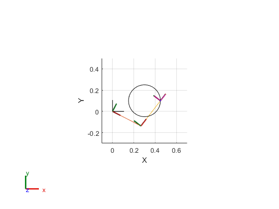
figure
show(robot,qs(1,:)');
view(2)
ax = gca;
ax.Projection = 'orthographic';
hold on
plot(points(:,1),points(:,2))
axis([-0.1 0.7 -0.3 0.5 -0.2 0.2])
Set up a rateControl object to display the robot trajectory at a fixed rate of 15 frames per second. Show the robot in each configuration from the inverse kinematic solver. Watch as the arm traces the circular trajectory shown.
framesPerSecond = 15;
r = rateControl(framesPerSecond);
for i = 1:count
    show(robot,qs(i,:)','PreservePlot',false);
    drawnow
    waitfor(r);
end

See Also
rigidBodyTree | rigidBody | rigidBodyJoint | inverseKinematics