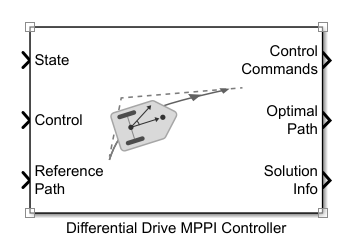
Differential Drive MPPI Controller

Control motion planning of differential drive vehicle model using Model Predictive Path Integral (MPPI)

Since R2025a

• 

Libraries:
Offroad Autonomy Library / Vehicle Controllers

Description

The Differential Drive MPPI Controller block enables you to plan a local path for a Differential Drive Kinematic Model, following a reference path typically generated by a global path planner such as RRT* or Hybrid A*, using the model predictive path integral (MPPI) algorithm.

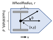
This model approximates a vehicle with single fixed axle and wheels separated by the track width specified in the Track Width parameter. Each wheel can be driven independently using speed inputs specified in the Vehicle Input Type parameter for the left and right wheels, respectively. Vehicle speed and heading are defined from the axle center.

At each state of the vehicle along the reference path, the MPPI controller samples potential trajectories for a short segment along the reference path, based on the current state and control of the vehicle. The controller evaluates these trajectories using a cost function to smooth the path and chooses an optimal trajectory and optimal control for the vehicle.

Examples

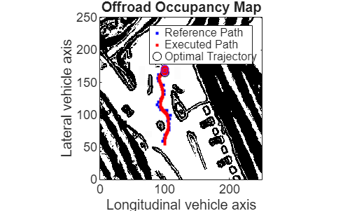
Plan Path Using Differential Drive MPPI Controller in Simulink

This example demonstrates how to follow an obstacle-free path with a differential drive vehicle model between two locations on a given map in Simulink®. It uses the RRT* planning algorithm to generate the path and the Differential Drive MPPI Controller block to generate control commands for navigating this path. It then simulates the vehicle motion based on those commands using a differential drive kinematic motion model.

Load Occupancy Map

Load the occupancy map, which defines the map limits and obstacles within the environment. This example uses the offroadMap in the exampleHelperPlotMap function.

exampleHelperPlotMap();

The exampleHelperPlotMap function is a utility that loads an occupancy map from a .mat file, such as occupancyMapData.mat, creates a binaryOccupancyMap object, and visualizes it using the plot function. This visualization allows users and developers to verify the environment in which the robot will navigate.

Specify a start and end location within the map.

startLoc = [2 2];
goalLoc = [18 15];

Open Simulink Model

Open the Simulink model to understand its structure.

open_system('pathPlanningDifferentialDriveMPPI.slx');

The model consists of three primary parts:

Planning: The Planner MATLAB Function block implements the RRT* algorithm. It takes the start location, goal location, and map as inputs, then outputs an array of waypoints that guide the vehicle to the goal position.

Path Following: This part consists of two key components:

• Differential Drive MPPI Controller: The Differential Drive MPPI Controller generates the linear and angular velocity commands based on the waypoints and the current vehicle pose.

• Has Reached Goal Flag: The HasReachedGoal flag, output by the Differential Drive MPPI Controller block within the Solution Info bus, indicates whether the vehicle has successfully reached the goal. This example uses this flag to stop the simulation upon reaching the goal.

Plant Model: The Plant Model simulates the simplified kinematics of the differential drive model, applying the velocity commands to drive the system's motion toward the goal.

Visualization: Displays the real-time behavior of the vehicle on the map, including its trajectory and current position.

The Visualization block in the model displays the real-time motion of the vehicle as it navigates the map. It dynamically updates the vehicle's trajectory and position while overlaying the start and goal locations on the occupancy map. The visualization leverages helper functions, such as exampleHelperVisualizeVehicle and exampleHelperVehicleGeometry, to ensure accurate rendering of the vehicle's dimensions and movements.

Run Simulink Model

Visualize the motion of the vehicle as it navigates the map using the simulation results.

simulation = sim('pathPlanningDifferentialDriveMPPI.slx');

Ports

Input

State — Pose of vehicle

three-element vector

Current position and orientation of the vehicle, specified as a [x y theta] vector, in meters and radians.

Data Types: double

Control — Current control commands of vehicle

two-element vector

Current control commands of the vehicle, specified as a two-element numeric vector, where the form depends on the motion model specified in the parameter Vehicle Input Type on the Vehicle tab.

For differential drive vehicle model motion, these values specified in the Vehicle Input Type parameter determine the format of the control command:

• Wheel Speeds — [wheelL wheelR]

• Vehicle Speed & Heading Angular Velocity — [v omegaDot]

v is the vehicle velocity in the direction of motion in meters per second. omegaDot is the angular velocity at the rear axle in radians per second. wheelL and wheelR are the left and right wheel speeds in radians per second, respectively.

Data Types: double

Reference Path — Reference path to follow

N-by-3 matrix

Reference path to follow, specified as an N-by-3 matrix in which each row represents a pose on the path.

Data Types: double

Wheel Speed Range — Minimum and maximum vehicle wheel speeds

[-2, 100] (default) | two-element vector

The steering rate range is a two-element vector that provides the minimum and maximum vehicle wheel speeds, [MinSpeed MaxSpeed], specified in radians per second.

Dependencies

To enable this port, select the Specify Wheel Speed (rad/s) Range from input port parameter on the Vehicle tab.

Data Types: double

Output

Control Commands — Optimal control command of vehicle

1-by-2 row matrix

Optimal control command of the vehicle, returned as an 1-by-2 matrix. The row of the matrix corresponds to the optimal control of the vehicle for a state along the trajectory. Each column depends on the motion model specified in the Vehicle Input Type parameter on the Vehicle tab.

For differential drive vehicle model motion, these values specified in the Vehicle Input Type parameter determine the format of the control command:

• Wheel Speeds — [wheelL wheelR]

• Vehicle Speed & Heading Angular Velocity — [v omegaDot]

v is the vehicle velocity in the direction of motion in meters per second. omegaDot is the angular velocity at the rear axle in radians per second. wheelL and wheelR are the left and right wheel speeds in radians per second, respectively.

Data Types: double

Optimal Path — Optimal path of vehicle

N-by-3 matrix

Optimal path of the differential drive vehicle model, returned as an N-by-3 matrix, where each row is in the form [x y θ].

N is the number of states along the trajectory. x is the current x-coordinate in meters. y is the current y-coordinate in meters. θ is the current heading angle of the vehicle in radians. Each row of the matrix corresponds to the optimal state of the vehicle for a state along the path.

Data Types: double

Solution Info — Extra information

scalar (bus)

Extra information, returned as a scalar (bus) with these fields.

Field	Description
HasReachedGoal	Indicates whether the vehicle has successfully reached the last pose of the reference path within the goal tolerance, returned as true if successful. Otherwise, this value is false.
ExitFlag	Scalar value indicating the exit condition. 0 — The control sequences and trajectories of the output are feasible. 1 — The control sequences and trajectories of the output are not feasible due to constraint violations. 2 — The next reference path pose is farther than what the vehicle can cover in the specified lookahead time while traveling at the maximum forward velocity of the vehicle model.

Data Types: bus

Parameters

To edit block parameters interactively, use the Property Inspector. From the Simulink^® Toolstrip, on the Simulation tab, in the Prepare gallery, select Property Inspector.

General

Configure various path-following parameters that guide the controller to make the vehicle accurately follow the desired path.

Path Following Parameters

Goal Tolerance — Tolerance around goal pose

[1 1 0.1] (default) | three-element vector

Tolerance around the goal pose, specified as a three-element vector of the form [x y θ]. x and y denote the position of the robot in the x- and y-directions, respectively. Units are in meters. θ is the heading angle of the robot in radians. This value specifies the maximum distance from the goal pose at which the planner can consider the robot to have reached the goal pose.

Lookahead Time — Lookahead time for trajectory planning in seconds

4 (default) | positive numeric scalar

Lookahead time for trajectory planning in seconds, specified as a positive numeric scalar.

The vehicle model determines the maximum forward velocity of the vehicle. The lookahead time of the controller multiplied by the maximum forward velocity of the vehicle determines the lookahead distance of the controller.

The lookahead distance of the controller is the distance from the current pose of the vehicle for which the controller must optimize the local path. The lookahead distance determines the segment of the global reference path from the current pose that the controller considers for an iteration of local path planning. The reference path pose at a lookahead distance from the current pose is the lookahead point, and all reference path poses between the current pose and the lookahead point are lookahead poses.

Increasing the value of lookahead time causes the controller to generate controls further into the future, enabling the vehicle to react earlier to unseen obstacles at the cost of increased computation time. Conversely, a smaller lookahead time reduces the available time to react to new unknown obstacles, but enables the controller to run at a faster rate.

Block Parameters

Sample Time (s) — Time interval at which the block updates during simulation in seconds

0.1 (default) | numeric

Time interval at which the block updates during simulation in seconds, specified as a numeric value. Use a positive scalar for discrete execution, or -1 to inherit from upstream blocks. You must ensure consistency with other model components for optimal performance.

Simulate using — Type of simulation to run

Code generation (default) | Interpreted execution

Specify the type of simulation to run.

• Code generation –– Simulate model using generated C code. The first time you run a simulation, Simulink generates C code for the block. The C code is reused for subsequent simulations, as long as the model does not change.

• Interpreted execution –– Simulate model using the MATLAB^® interpreter. For more information, see Interpreted Execution vs. Code Generation (Simulink).

Tunable: No

Vehicle

Specify the vehicle specifications, limits, and other properties for a Differential Drive Kinematic Model.

Vehicle Specifications

Vehicle Input Type — Type of speed and directional inputs for vehicle

Wheel Speeds (default) | Vehicle Speed & Heading Angular Velocity

Format of the model input commands, specified as one of these options:

• Wheel Speeds — Angular speeds of the two wheels in radians per second.

• Vehicle Speed & Heading Angular Velocity — Vehicle speed in meters per second, with a heading angular velocity in radians per second.

Wheel Radius — Wheel radius of vehicle

0.05 (default) | positive numeric scalar

Radius of the wheels on the vehicle, specified in meters.

Track Width — Track length of vehicle from wheel to wheel

0.2 (default) | numeric scalar

Length of the track from the left wheel to right wheel, specified in meters.

Vehicle Limits

Wheel Speed Range (rad/s) — Minimum and maximum vehicle wheel speeds

[-2 100] (default) | two-element vector

The wheel speed range is a two-element vector that provides the minimum and maximum vehicle wheel speeds, [MinSpeed MaxSpeed], specified in radians per second.

Specify Vehicle Properties from Input Ports

Specify Wheel Speed (rad/s) Range from input port — Minimum and maximum vehicle wheel speeds

off (default) | on

Select this parameter to specify the wheel speed range of the differential drive vehicle model at the Wheel Speed Range input port. Enabling this option removes the Wheel Speed (rad/s) Range parameter from the block mask.

Controller

Specify various parameters for the MPPI controller, which is used for motion planning of the bicycle vehicle model in the Differential Drive MPPI Controller block.

Cost Weights

Path Alignment Weight — Weight for aligning with lookahead poses

1 (default) | nonnegative scalar

Weight for aligning with the lookahead poses of the reference path, specified as a nonnegative scalar.

Path Following Weight — Weight for closely following lookahead point

1 (default) | nonnegative scalar

Weight for closely following lookahead point, specified as a nonnegative scalar.

Control Smoothness Weight — Weight for smooth control actions

1 (default) | nonnegative scalar

Weight for smooth control actions, avoiding abrupt changes, specified as a nonnegative scalar.

Trajectory Generation Parameters

Number of trajectories — Number of sampled trajectories

500 (default) | positive integer

Number of sampled trajectories, specified as a positive integer.

The controller calculates the optimal trajectory by averaging the controls of candidate trajectories, with weights determined by their associated costs.

A larger number of trajectories can lead to a more thorough search of the trajectory space and a potentially better solution, at the cost of increased computation time.

Time Step (s) — Time between consecutive states of trajectory in seconds

0.1 (default) | positive scalar

Time between consecutive states of the trajectory in seconds, specified as a positive scalar. Smaller values lead to more precise trajectory predictions, but increased computation time.

Standard Deviation — Standard deviation for vehicle inputs

[0.5 0.5] (default) | two-element numeric vector

Standard deviation for vehicle inputs, specified as a two-element numeric vector with nonnegative values. For the differential drive vehicle model, the default value is [0.5 0.5].

Each element of the vector specifies the standard deviation for a control input of the vehicle model, such as steering or velocity. Each model has two control inputs. By introducing such variability into the control inputs during trajectory sampling, the controller can better explore different possible trajectories. Larger standard deviations enable the controller to account for uncertainties in the control input and achieve more realistic trajectory predictions.

Trajectory Selection Bias (λ) — Selectiveness of optimal trajectory

1000 (default) | positive scalar

Selectiveness of the optimal trajectory, specified as a positive scalar.

Specify a value close to 0 to favor the trajectory with the lowest cost as the optimal trajectory. Specify a larger value to favor the average of all sampled trajectories as the optimal trajectory.

This parameter adjusts the sensitivity of the MPPI algorithm to the cost differences, acting as a scaling factor that influences the weighting of candidate trajectories.

Extended Capabilities

C/C++ Code Generation
Generate C and C++ code using Simulink® Coder™.

Version History

Introduced in R2025a