modelDiscrimination
Syntax
Description
DiscMeasure = modelDiscrimination(lgdModel,data)modelDiscrimination supports segmentation and comparison
against a reference model and also alternative methods to discretize the LGD
response into a binary variable.
[
specifies options using one or more name-value pair arguments in addition to the
input arguments in the previous syntax.DiscMeasure,DiscData] = modelDiscrimination(___,Name,Value)
Examples
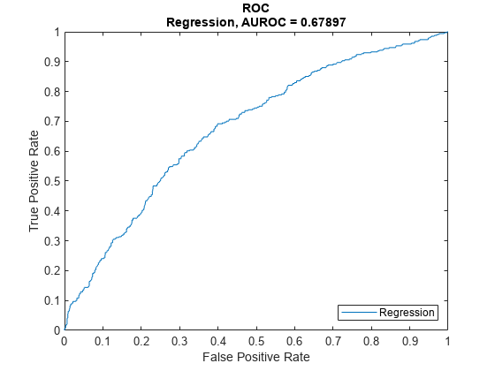
This example shows how to use fitLGDModel to fit data with a Regression model and then use modelDiscrimination to compute AUROC and ROC.
Load Data
Load the loss given default data.
load LGDData.mat
head(data)
LTV Age Type LGD
_______ _______ ___________ _________
0.89101 0.39716 residential 0.032659
0.70176 2.0939 residential 0.43564
0.72078 2.7948 residential 0.0064766
0.37013 1.237 residential 0.007947
0.36492 2.5818 residential 0
0.796 1.5957 residential 0.14572
0.60203 1.1599 residential 0.025688
0.92005 0.50253 investment 0.063182
Partition Data
Separate the data into training and test partitions.
rng('default'); % for reproducibility
NumObs = height(data);

c = cvpartition(NumObs,'HoldOut',0.4);
TrainingInd = training(c);
TestInd = test(c);
Create a Regression LGD Model
Use fitLGDModel to create a Regression model using training data. You can also use fitLGDModel to create a Tobit model by changing the lgdModel input argument to 'Tobit'.
lgdModel = fitLGDModel(data(TrainingInd,:),'Regression');
disp(lgdModel)
Regression with properties:
ResponseTransform: "logit"
BoundaryTolerance: 1.0000e-05
ModelID: "Regression"
Description: ""
UnderlyingModel: [1×1 classreg.regr.CompactLinearModel]
PredictorVars: ["LTV" "Age" "Type"]
ResponseVar: "LGD"
WeightsVar: ""
Display the underlying model.
disp(lgdModel.UnderlyingModel)
Compact linear regression model:
    LGD_logit ~ 1 + LTV + Age + Type

Estimated Coefficients:
                       Estimate       SE        tStat       pValue
                       ________    ________    _______    __________

    (Intercept)        -4.7549      0.36041    -13.193    3.0997e-38
    LTV                 2.8565      0.41777     6.8377    1.0531e-11
    Age                -1.5397     0.085716    -17.963    3.3172e-67
    Type_investment     1.4358       0.2475     5.8012     7.587e-09


Number of observations: 2093, Error degrees of freedom: 2089
Root Mean Squared Error: 4.24
R-squared: 0.206,  Adjusted R-Squared: 0.205
F-statistic vs. constant model: 181, p-value = 2.42e-104
Compute AUROC and ROC Data
Use modelDiscrimination to compute the AUROC and ROC for the test data set.
[DiscMeasure,DiscData] = modelDiscrimination(lgdModel,data(TestInd,:),'ShowDetails',true)DiscMeasure=1×4 table
AUROC Segment SegmentCount WeightedCount
_______ __________ ____________ _____________
Regression 0.67897 "all_data" 1394 1394
DiscData=1395×3 table
        X             Y           T
    __________    _________    _______

             0            0    0.87604
             0    0.0029326    0.87604
             0    0.0058651     0.7515
    0.00094967    0.0058651    0.44074
     0.0018993    0.0058651    0.43569
     0.0018993    0.0087977    0.40058
      0.002849    0.0087977    0.31703
      0.002849      0.01173    0.30375
      0.002849     0.014663    0.28789
      0.002849     0.017595    0.27996
     0.0037987     0.017595    0.27026
     0.0047483     0.017595    0.26868
      0.005698     0.017595    0.26854
      0.005698     0.020528    0.26682
     0.0066477     0.020528    0.26668
     0.0066477      0.02346    0.24923
      ⋮
You can visualize the ROC data using modelDiscriminationPlot.
modelDiscriminationPlot(lgdModel,data(TestInd,:))

This example shows how to use fitLGDModel to fit data with a Tobit model and then use modelDiscrimination to compute AUROC and ROC.
Load Data
Load the loss given default data.
load LGDData.mat
head(data)
LTV Age Type LGD
_______ _______ ___________ _________
0.89101 0.39716 residential 0.032659
0.70176 2.0939 residential 0.43564
0.72078 2.7948 residential 0.0064766
0.37013 1.237 residential 0.007947
0.36492 2.5818 residential 0
0.796 1.5957 residential 0.14572
0.60203 1.1599 residential 0.025688
0.92005 0.50253 investment 0.063182
Partition Data
Separate the data into training and test partitions.
rng('default'); % for reproducibility
NumObs = height(data);

c = cvpartition(NumObs,'HoldOut',0.4);
TrainingInd = training(c);
TestInd = test(c);
Create a Tobit LGD Model
Use fitLGDModel to create a Tobit model using training data.
lgdModel = fitLGDModel(data(TrainingInd,:),'tobit');
disp(lgdModel)
Tobit with properties:
CensoringSide: "both"
LeftLimit: 0
RightLimit: 1
Weights: [0×1 double]
ModelID: "Tobit"
Description: ""
UnderlyingModel: [1×1 risk.internal.credit.TobitModel]
PredictorVars: ["LTV" "Age" "Type"]
ResponseVar: "LGD"
WeightsVar: ""
Display the underlying model.
disp(lgdModel.UnderlyingModel)
Tobit regression model:
     LGD = max(0,min(Y*,1))
     Y* ~ 1 + LTV + Age + Type

Estimated coefficients:
                       Estimate        SE         tStat       pValue
                       _________    _________    _______    __________

    (Intercept)         0.058257      0.02728     2.1355      0.032837
    LTV                  0.20126     0.031373      6.415    1.7363e-10
    Age                -0.095407     0.007258    -13.145             0
    Type_investment      0.10208     0.018076     5.6472     1.853e-08
    (Sigma)              0.29288    0.0057084     51.307             0

Number of observations: 2093
Number of left-censored observations: 547
Number of uncensored observations: 1521
Number of right-censored observations: 25
Log-likelihood: -698.383
Compute AUROC and ROC Data
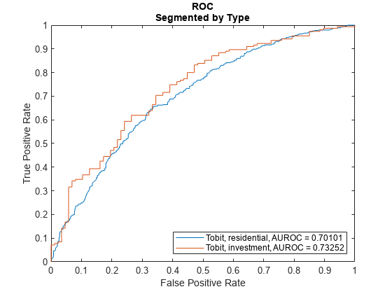
Use modelDiscrimination to compute the AUROC and ROC for the test data set.
DiscMeasure = modelDiscrimination(lgdModel,data(TestInd,:),'ShowDetails',true,'SegmentBy',"Type",'DiscretizeBy',"median")
DiscMeasure=2×4 table
                                AUROC        Segment       SegmentCount    WeightedCount
                               _______    _____________    ____________    _____________

    Tobit, Type=residential    0.70101    "residential"        1152            1152
    Tobit, Type=investment     0.73252    "investment"          242             242
You can visualize the ROC using modelDiscriminationPlot.
modelDiscriminationPlot(lgdModel,data(TestInd,:),'SegmentBy',"Type",'DiscretizeBy',"median")

This example shows how to use fitLGDModel to fit data with a Beta model and then use modelDiscrimination to compute AUROC and ROC.
Load Data
Load the loss given default data.
load LGDData.mat
head(data)
LTV Age Type LGD
_______ _______ ___________ _________
0.89101 0.39716 residential 0.032659
0.70176 2.0939 residential 0.43564
0.72078 2.7948 residential 0.0064766
0.37013 1.237 residential 0.007947
0.36492 2.5818 residential 0
0.796 1.5957 residential 0.14572
0.60203 1.1599 residential 0.025688
0.92005 0.50253 investment 0.063182
Partition Data
Separate the data into training and test partitions.
rng('default'); % for reproducibility
NumObs = height(data);

c = cvpartition(NumObs,'HoldOut',0.4);
TrainingInd = training(c);
TestInd = test(c);
Create a Beta LGD Model
Use fitLGDModel to create a risk_ug#object_model_beta_lgd model using training data.
lgdModel = fitLGDModel(data(TrainingInd,:),'Beta');
disp(lgdModel)
Beta with properties:
BoundaryTolerance: 1.0000e-05
ModelID: "Beta"
Description: ""
UnderlyingModel: [1×1 risk.internal.credit.BetaModel]
PredictorVars: ["LTV" "Age" "Type"]
ResponseVar: "LGD"
WeightsVar: ""
Display the underlying model.
disp(lgdModel.UnderlyingModel)
Beta regression model:
     logit(LGD) ~ 1_mu + LTV_mu + Age_mu + Type_mu
     log(LGD) ~ 1_phi + LTV_phi + Age_phi + Type_phi

Estimated coefficients:
                           Estimate       SE        tStat       pValue
                           ________    ________    _______    __________

    (Intercept)_mu          -1.3772     0.13201    -10.433             0
    LTV_mu                   0.6027     0.15087     3.9948    6.6993e-05
    Age_mu                 -0.47464    0.040264    -11.788             0
    Type_investment_mu      0.45372    0.085143     5.3289    1.0941e-07
    (Intercept)_phi        -0.16336     0.12591    -1.2974       0.19462
    LTV_phi                0.055886     0.14719    0.37969       0.70421
    Age_phi                 0.22887    0.040335     5.6743     1.586e-08
    Type_investment_phi    -0.14102    0.078155    -1.8044      0.071313

Number of observations: 2093
Log-likelihood: -5291.04
Compute AUROC and ROC Data
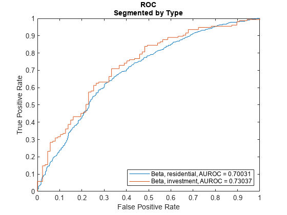
Use modelDiscrimination to compute the AUROC and ROC for the test data set.
DiscMeasure = modelDiscrimination(lgdModel,data(TestInd,:),'ShowDetails',true,'SegmentBy',"Type",'DiscretizeBy',"median")
DiscMeasure=2×4 table
                               AUROC        Segment       SegmentCount    WeightedCount
                              _______    _____________    ____________    _____________

    Beta, Type=residential    0.70031    "residential"        1152            1152
    Beta, Type=investment     0.73037    "investment"          242             242
You can visualize the ROC using modelDiscriminationPlot.
modelDiscriminationPlot(lgdModel,data(TestInd,:),'SegmentBy',"Type",'DiscretizeBy',"median")

Input Arguments
Loss given default model, specified as a previously created Regression,
Tobit, or Beta object using
fitLGDModel.
Data Types: object
Data, specified as a
NumRows-by-NumCols table with
predictor and response values. The variable names and data types must be
consistent with the underlying model.
Data Types: table
Name-Value Arguments
Specify optional pairs of arguments as
Name1=Value1,...,NameN=ValueN, where Name is
the argument name and Value is the corresponding value.
Name-value arguments must appear after other arguments, but the order of the
pairs does not matter.
Before R2021a, use commas to separate each name and value, and enclose
Name in quotes.
Example: [DiscMeasure,DiscData] =
modelDiscrimination(lgdModel,data(TestInd,:),'DataID','Testing','DiscretizeBy','median')
Data set identifier, specified as the comma-separated pair consisting
of 'DataID' and a character vector or string. The
DataID is included in the output for reporting
purposes.
Data Types: char | string
Discretization method for LGD data, specified as
the comma-separated pair consisting of 'DiscretizeBy'
and a character vector or string.
'mean'— Discretized response is1if observed LGD is greater than or equal to the mean LGD,0otherwise.'median'— Discretized response is1if observed LGD is greater than or equal to the median LGD,0otherwise.'positive'— Discretized response is1if observed LGD is positive,0otherwise (full recovery).'total'— Discretized response is1if observed LGD is greater than or equal to1(total loss),0otherwise.
Data Types: char | string
Name of a column in the data input, not
necessarily a model variable, to be used to segment the data set,
specified as the comma-separated pair consisting of
'SegmentBy' and a character vector or string. One
AUROC is reported for each segment, and the corresponding ROC data for
each segment is returned in the optional output.
Data Types: char | string
Since R2022a
Indicates if the output includes columns showing segment value and
segment count, specified as the comma-separated pair consisting of
'ShowDetails' and a scalar logical.
Data Types: logical
Identifier for the reference model, specified as the comma-separated
pair consisting of 'ReferenceID' and a character
vector or string. 'ReferenceID' is used in the
modelDiscrimination output for reporting
purposes.
Data Types: char | string
Output Arguments
AUROC information for each model and each segment, returned as a table.
DiscMeasure has a single column named
'AUROC' and the number of rows depends on the number
of segments and whether you use a ReferenceID for a
reference model. The row names of DiscMeasure report the
model IDs, segment, and data ID. If the optional
ShowDetails name-value argument is
true, the DiscMeasure output
displays Segment, SegmentCount, and
WeightedCount columns.
Note
If you do not specify SegmentBy and use
ShowDetails to request the segment details,
the two columns are added and show the Segment
column as "all_data" and the sample size (minus
missing values) for the SegmentCount
column.
ROC data for each model and each segment, returned as a table. There are
three columns for the ROC data, with column names 'X',
'Y', and 'T', where the first two
are the X and Y coordinates of the ROC curve, and T contains the
corresponding thresholds. For more information, see Model Discrimination or perfcurve.
If you use SegmentBy, the function stacks the ROC
data for all segments and DiscData has a column with the
segmentation values to indicate where each segment starts and ends.
If reference model data is given, the DiscData outputs
for the main and reference models are stacked, with an extra column
'ModelID' indicating where each model starts and
ends.
More About
Model discrimination measures the risk ranking.
The modelDiscrimination function computes the area under the
receiver operator characteristic (AUROC) curve, sometimes called simply the area
under the curve (AUC). This metric is between 0 and 1 and higher values indicate
better discrimination.
To compute the AUROC, you need a numeric prediction and a binary response. For
loss given default (LGD) models, the predicted LGD is used directly as the
prediction. However, the observed LGD must be discretized into a binary variable. By
default, observed LGD values greater than or equal to the mean observed LGD are
assigned a value of 1, and values below the mean are assigned a value of 0. This
discretized response is interpreted as "high LGD" vs. "low LGD." Therefore, the
modelDiscrimination function measures how well the predicted
LGD separates the "high LGD" vs. the "low LGD" observations. You can change the
discretization criterion with the DiscretizeBy name-value pair
argument.
To plot the receiver operator characteristic (ROC) curve, use the modelDiscriminationPlot function. However, if the ROC curve data is
needed, use the optional DiscData output argument from the
modelDiscrimination function.
The ROC curve is a parametric curve that plots the proportion of
High LGD cases with predicted LGD greater than or equal to a parameter t, or true positive rate (TPR)
Low LGD cases with predicted LGD greater than or equal to the same parameter t, or false positive rate (FPR)
The parameter t sweeps through all the observed predicted LGD
values for the given data. The DiscData optional output
contains the TPR in the 'X' column, the FPR in the
'Y' column, and the corresponding parameters
t in the 'T' column. For more information
about ROC curves, see ROC Curve and Performance Metrics.
If the LGD model object is created by using the WeightsVar
name-value argument, the AUROC and ROC are weighted quantities.
References
[1] Baesens, Bart, Daniel Roesch, and Harald Scheule. Credit Risk Analytics: Measurement Techniques, Applications, and Examples in SAS. Wiley, 2016.
[2] Bellini, Tiziano. IFRS 9 and CECL Credit Risk Modelling and Validation: A Practical Guide with Examples Worked in R and SAS. San Diego, CA: Elsevier, 2019.
Version History
Introduced in R2021aThe DiscMeasure output supports an additional column for
WeightedCount.
The lgdModel input supports an option for a
Beta model object that you can create using fitLGDModel.
There is an additional name-value pair for ShowDetails to
indicate if the DiscMeasure output includes columns for
Segment value and the SegmentCount.
See Also
Tobit | Regression | modelCalibration | modelCalibrationPlot | modelDiscriminationPlot | predict | fitLGDModel
MATLAB Command
You clicked a link that corresponds to this MATLAB command:
Run the command by entering it in the MATLAB Command Window. Web browsers do not support MATLAB commands.
Select a Web Site
Choose a web site to get translated content where available and see local events and offers. Based on your location, we recommend that you select: .
You can also select a web site from the following list
How to Get Best Site Performance
Select the China site (in Chinese or English) for best site performance. Other MathWorks country sites are not optimized for visits from your location.
Americas
- América Latina (Español)
- Canada (English)
- United States (English)
Europe
- Belgium (English)
- Denmark (English)
- Deutschland (Deutsch)
- España (Español)
- Finland (English)
- France (Français)
- Ireland (English)
- Italia (Italiano)
- Luxembourg (English)
- Netherlands (English)
- Norway (English)
- Österreich (Deutsch)
- Portugal (English)
- Sweden (English)
- Switzerland
- United Kingdom (English)