phased.URA
Uniform rectangular array
Description
To create a Uniform Rectangular Array (URA) System object™:
Create the
phased.URAobject and set its properties.Call the object with arguments, as if it were a function.
To learn more about how System objects work, see What Are System Objects?
Creation
Description
array = phased.URAarray (URA) System object that models a URA formed from identical isotropic phased array elements.
Array elements are contained in the yz-plane in a
rectangular lattice. The array look direction (boresight) points along the positive
x-axis.
array = phased.URA(Name=Value)array object with each specified property Name set to the
specified Value. You can specify additional name-value pair arguments in any order as
(Name1=Value1, ...,
NameN=ValueN). All properties needed to fully
specify this object can be found in Properties.Response of 2-by-2 URA of Short-Dipole Antennas.
array = phased.URA(SZ,D,Name=Value)phased.URA
array
System object with its Size property set to SZ
and its ElementSpacing property set to D. Other
specified property Names are set to the specified Values. SZ and
D are value-only arguments. When specifying a value-only argument,
specify all preceding value-only arguments. You can specify name-value pair arguments in
any order.
Properties
Unless otherwise indicated, properties are nontunable, which means you cannot change their
values after calling the object. Objects lock when you call them, and the
release function unlocks them.
If a property is tunable, you can change its value at any time.
For more information on changing property values, see System Design in MATLAB Using System Objects.
Phased array element, specified as a Phased Array System Toolbox antenna, microphone, or transducer element or Antenna Toolbox antenna.
Example: phased.CosineAntennaElement
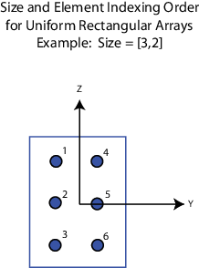
Array size, specified as a 1-by-2 vector of integers or a single integer. containing
the size of the array. If Size is a 1-by-2 vector, the vector has
the form [NumberOfRows, NumberOfColumns]. If
Size is a scalar, the array has the same number of elements in
each row and column. For a URA, array elements are indexed from top to bottom along a
column and continuing to the next columns from left to right. In this illustration, a
Size value of [3,2] array has three rows and
two columns.
Example: [3,2]
Data Types: double
Element spacing, specified as a positive scalar or 1-by-2 vector of positive values.
If ElementSpacing is a 1-by-2 vector, it has the form
[SpacingBetweenRows,SpacingBetweenColumns]. See Spacing Between Columns and Spacing Between Rows. If ElementSpacing is a scalar,
both row and column spacings are equal. Units are in meters.
Example: [0.3, 0.5]
Data Types: double
Element lattice type, specified as "Rectangular" or
"Triangular". When you set the Lattice
property to "Rectangular", all elements of the URA are aligned in
both row and column directions. When you set the Lattice property
to "Triangular", elements in even rows are displaced toward the
positive row axis direction. The displacement is one-half the element spacing along the
row.
Example: "Triangular"
Data Types: char | string
Array normal direction, specified as one of "x", "y", or
"z". URA elements lie in a plane orthogonal to the selected array
normal direction. Element boresight directions point along the array normal
direction.
| ArrayNormal Property Value | Element Positions and Boresight Directions |
|---|---|
"x" | Array elements lie on the yz-plane. All element boresight vectors point along the x-axis. This is the default value. |
"y" | Array elements lie on the zx-plane. All element boresight vectors point along the y-axis. |
"z" | Array elements lie on the xy-plane. All element boresight vectors point along the z-axis. |
Element tapers, specified as a complex-valued scalar, complex-valued
1-by-MN vector, or complex-valued
M-by-N matrix. Tapers are applied to each
element in the sensor array. Tapers are often referred to as element
weights. M is the number of elements along
the z-axis, and N is the number of elements along
y-axis. M and N correspond to
the values of [NumberofRows,NumberOfColumns] in the
SIze property. If Taper is a scalar, the same
taper value is applied to all elements. If the value of Taper is a
vector or matrix, taper values are applied to the corresponding elements. Tapers are
used to modify both the amplitude and phase of the received data.
Example: [0.4 1 0.4]
Data Types: double
Usage
Syntax
Description
RESP = array(FREQ,ANG)RESP, at the operating
frequencies specified in FREQ and directions specified in
ANG.
Note
The object performs an initialization the first time the object is executed. This
initialization locks nontunable properties
and input specifications, such as dimensions, complexity, and data type of the input data.
If you change a nontunable property or an input specification, the System object issues an error. To change nontunable properties or inputs, you must first
call the release method to unlock the object.
Input Arguments
Output Arguments
Object Functions
To use an object function, specify the
System object as the first input argument. For
example, to release system resources of a System object named obj, use
this syntax:
release(obj)
Examples
Construct a 2-by-2 rectangular lattice URA of short-dipole antenna elements. Then, find the response of each element at boresight. Assume the operating frequency is 1 GHz.
sSD = phased.ShortDipoleAntennaElement;
sURA = phased.URA(Element=sSD,Size=[2 2]);
fc = 1e9;
ang = [0;0];
resp = sURA(fc,ang);
disp(resp.V)
   -1.2247
   -1.2247
   -1.2247
   -1.2247
Construct a 3-by-2 rectangular lattice URA. By default, the array consists of isotropic antenna elements. Find the response of each element at boresight, 0° azimuth and elevation. Assume the operating frequency is 1 GHz.
array = phased.URA(Size=[3 2]);
fc = 1e9;
ang = [0;0];
resp = array(fc,ang);
disp(resp)
     1
     1
     1
     1
     1
     1
Plot the azimuth pattern of the array.
c = physconst("LightSpeed");
pattern(array,fc,[-180:180],0,PropagationSpeed=c, ...
    CoordinateSystem="polar",Type="powerdb",Normalize=true)

This example shows how to find and plot the positions of the elements of a 5-row-by-6-column URA with a triangular lattice and a URA with a rectangular lattice. The element spacing is 0.5 meters for both lattices.
Create the arrays.
h_tri = phased.URA(Size=[5 6],Lattice="Triangular");
h_rec = phased.URA(Size=[5 6],Lattice="Rectangular");
Get the element y,z positions for each array. All the x coordinates are zero.
pos_tri = getElementPosition(h_tri);
pos_rec = getElementPosition(h_rec);
pos_yz_tri = pos_tri(2:3,:);
pos_yz_rec = pos_rec(2:3,:);
Plot the element positions in the yz-plane.
figure;
gcf.Position = [100 100 300 400];
subplot(2,1,1);
plot(pos_yz_tri(1,:), pos_yz_tri(2,:), '.')
axis([-1.5 1.5 -2 2])
xlabel("y"); ylabel("z")
title("Triangular Lattice")
subplot(2,1,2);
plot(pos_yz_rec(1,:), pos_yz_rec(2,:), '.')
axis([-1.5 1.5 -2 2])
xlabel("y"); ylabel("z")
title("Rectangular Lattice")

Construct a 5-by-2 element URA with a Taylor window taper along each column. The tapers form a 5-by-2 matrix.
taper = taylorwin(5);
ha = phased.URA([5,2],Taper=[taper,taper]);
w = getTaper(ha)
w = 10×1

    0.5181
    1.2029
    1.5581
    1.2029
    0.5181
    0.5181
    1.2029
    1.5581
    1.2029
    0.5181
Simulate two received random signals at a 6-element URA. The array has a rectangular lattice with two elements in the row direction and three elements in the column direction. The signals arrive from 10° and 30° azimuth. Both signals have an elevation angle of 0°. Assume the propagation speed is the speed of light and the carrier frequency of the signal is 100 MHz.
array = phased.URA([2 3]);
fc = 100e6;
y = collectPlaneWave(array,randn(4,2),[10 30],fc,physconst("LightSpeed"));Compute the directivity of two uniform rectangular arrays (URA). The first array consists of isotropic antenna elements. The second array consists of cosine antenna elements. In addition, compute the directivity of the first array steered to a specific direction.
Array of Isotropic Antenna Elements
First, create a 10-by-10-element URA of isotropic antenna elements spaced one-quarter wavelength apart. Set the signal frequency to 800 MHz.
c = physconst("LightSpeed");
fc = 3e8;
lambda = c/fc;
myAntIso = phased.IsotropicAntennaElement;
myArray1 = phased.URA;
myArray1.Element = myAntIso;
myArray1.Size = [10,10];
myArray1.ElementSpacing = [lambda*0.25,lambda*0.25];
ang = [0;0];
d = directivity(myArray1,fc,ang,PropagationSpeed=c)
d = 15.7753
Array of Cosine Antenna Elements
Next, create a 10-by-10-element URA of cosine antenna elements also spaced one-quarter wavelength apart.
myAntCos = phased.CosineAntennaElement(CosinePower=[1.8,1.8]);
myArray2 = phased.URA;
myArray2.Element = myAntCos;
myArray2.Size = [10,10];
myArray2.ElementSpacing = [lambda*0.25,lambda*0.25];
ang = [0;0];
d = directivity(myArray2,fc,ang,PropagationSpeed=c)
d =
19.7295
The directivity is increased due to the directivity of the cosine antenna elements.
Steered Array of Isotropic Antenna Elements
Finally, steer the isotropic antenna array to 30 degrees in azimuth and examine the directivity at the steered angle.
ang = [30;0];
w = steervec(getElementPosition(myArray1)/lambda,ang);
d = directivity(myArray1,fc,ang,PropagationSpeed=c, ...
    Weights=w)
d = 15.3309
The directivity is maximum in the steered direction and equals the directivity of the unsteered array at boresight.
Construct three 2-by-2 URA's with element normals along the x-, y-, and z-axes. Obtain the element positions and normal directions.
First, choose the array normal along the x-axis.
sURA1 = phased.URA(Size=[2,2],ArrayNormal="x");
pos = getElementPosition(sURA1)
pos = 3×4
0 0 0 0
-0.2500 -0.2500 0.2500 0.2500
0.2500 -0.2500 0.2500 -0.2500
normvec = getElementNormal(sURA1)
normvec = 2×4
0 0 0 0
0 0 0 0
All elements lie in the yz-plane and the element normal vectors point along the x-axis (0°,0°).
Next, choose the array normal along the y-axis.
sURA2 = phased.URA(Size=[2,2],ArrayNormal="y");
pos = getElementPosition(sURA2)pos = 3×4
0.2500 0.2500 -0.2500 -0.2500
0 0 0 0
0.2500 -0.2500 0.2500 -0.2500
normvec = getElementNormal(sURA2)
normvec = 2×4
90 90 90 90
0 0 0 0
All elements lie in the zx-plane and the element normal vectors point along the y-axis (90°,0°).
Finally, set the array normal along the z-axis. Obtain the normal vectors of the odd-numbered elements.
sURA3 = phased.URA(Size=[2,2],ArrayNormal="z");
pos = getElementPosition(sURA3)pos = 3×4
-0.2500 -0.2500 0.2500 0.2500
0.2500 -0.2500 0.2500 -0.2500
0 0 0 0
normvec = getElementNormal(sURA3,[1,3])
normvec = 2×2
0 0
90 90
All elements lie in the xy-plane and the element normal vectors point along the z-axis (0°,90°).
Construct a default URA with a rectangular lattice, and obtain the element positions.
array = phased.URA; pos = getElementPosition(array)
pos = 3×4

         0         0         0         0
   -0.2500   -0.2500    0.2500    0.2500
    0.2500   -0.2500    0.2500   -0.2500
Construct a default URA, and obtain the number of elements.
array = phased.URA;
N = getNumElements(array)
N =
4
Construct a 5-by-2 element URA with a Taylor window taper along each column. Then, draw the array showing the element taper shading.
taper = taylorwin(5);
array = phased.URA([5,2],Taper=[taper,taper]);
w = getTaper(array)
w = 10×1

    0.5181
    1.2029
    1.5581
    1.2029
    0.5181
    0.5181
    1.2029
    1.5581
    1.2029
    0.5181
viewArray(array,ShowTaper=true)

Show that a URA array of phased.ShortDipoleAntennaElement short-dipole antenna elements supports polarization.
antenna = phased.ShortDipoleAntennaElement(FrequencyRange=[1e9 10e9]);
array = phased.URA([3,2],Element=antenna);
isPolarizationCapable(array)
ans = logical
   1
The returned value 1 shows that this array supports polarization.
Create a 5x7-element URA operating at 1 GHz. Assume the elements are spaced one-half wavelength apart. Show the 3-D array patterns.
Create the Array
sSD = phased.ShortDipoleAntennaElement(...
    FrequencyRange=[50e6,1000e6], ...
    AxisDirection="Z");
fc = 500e6;
c = physconst("LightSpeed");
lam = c/fc;
sURA = phased.URA(Element=sSD, ...
    Size=[5,7], ...
    ElementSpacing=0.5*lam);
Evaluate the fields of the first five elements at 45° azimuth and 0° elevation.
ang = [45;0];
resp = sURA(fc,ang);
disp(resp.V(1:5))
   -1.2247
   -1.2247
   -1.2247
   -1.2247
   -1.2247
Display the 3-D Directivity Pattern at 500 MHz in Polar Coordinates
pattern(sURA,fc,[-180:180],[-90:90], ...
    CoordinateSystem="polar", ...
    Type="directivity",PropagationSpeed=c)

Display the 3-D Directivity Pattern at 500 MHz in UV Coordinates
pattern(sURA,fc,[-1.0:.01:1.0],[-1.0:.01:1.0], ...
    CoordinateSystem="uv", ...
    Type="directivity",PropagationSpeed=c)

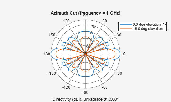
Create a 5x7-element URA of short-dipole antenna elements operating at 1 GHz. Assume the elements are spaced one-half wavelength apart. Plot the array azimuth directivity patterns for two different elevation angles, 0° and 15°. The patternAzimuth method always plots the array pattern in polar coordinates.
Create the Array
sSD = phased.ShortDipoleAntennaElement(...
    FrequencyRange=[50e6,1000e6], ...
    AxisDirection="Z");
fc = 1e9;
c = physconst("LightSpeed");
lam = c/fc;
sURA = phased.URA(Element=sSD, ...
    Size=[5,7], ...
    ElementSpacing=0.5*lam);
Display the Pattern
Display the azimuth directivity pattern at 1 GHz in polar coordinates
patternAzimuth(sURA,fc,[0 15], ...
    PropagationSpeed=c, ...
    Type="directivity")
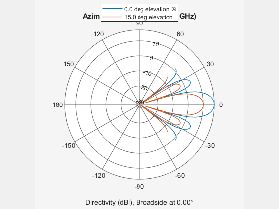
Display a Subset of Angles
You can plot a smaller range of azimuth angles by setting the Azimuth parameter.
patternAzimuth(sURA,fc,[0 15], ...
    PropagationSpeed=c, ...
    Type="directivity", ...
    Azimuth=[-45:45])
Create a 7x7-element URA of backbaffled omnidirectional transducer elements operating at 1 kHz. Assume the speed of sound in water is 1500 m/s. The elements are spaced less than one-half wavelength apart. Plot the array elevation directivity patterns for three different azimuth angles, -20°, 0°, and 15°. The patternElevation method always plots the array pattern in polar coordinates.
Create the Array
element = phased.OmnidirectionalMicrophoneElement(...
    FrequencyRange=[20,3000], ...
    BackBaffled=true);
fc = 1000;
c = 1500;
lam = c/fc;
array = phased.URA(Element=element, ...
    Size=[7,7], ...
    ElementSpacing=0.45*lam);
Display the Pattern
Display the azimuth directivity pattern at 1 GHz in polar coordinates.
patternElevation(array,fc,[-20, 0, 15], ...
    PropagationSpeed=c,...
    Type="directivity")

Display a Subset of Elevation Angles
You can plot a smaller range of elevation angles by setting the Elevation parameter.
patternElevation(array,fc,[-20, 0, 15], ...
    PropagationSpeed=c, ...
    Type="directivity", ...
    Elevation=[-45:45])

Plot the grating lobe diagram for an 11-by-9-element uniform rectangular array having element spacing equal to one-half wavelength.
Assume the operating frequency of the array is 10 kHz. All elements are omnidirectional microphone elements. Steer the array in the direction 20° in azimuth and 30° in elevation. The speed of sound in air is 344.21 m/s at 21° C.
cair = 344.21;
f = 10.0e3;
lambda = cair/f;
microphone = phased.OmnidirectionalMicrophoneElement(...
    FrequencyRange=[20 20000]);
array = phased.URA(Element=microphone,Size=[11,9], ...
    ElementSpacing=0.5*lambda*[1,1]);
plotGratingLobeDiagram(array,f,[20;30],cair);

Plot the grating lobes. The main lobe of the array is indicated by a filled black circle. The grating lobes in visible and nonvisible regions are indicated by unfilled black circles. The visible region is the region in u-v coordinates for which . The visible region is shown as a unit circle centered at the origin. Because the array spacing is less than one-half wavelength, there are no grating lobes in the visible region of space. There are an infinite number of grating lobes in the nonvisible regions, but only those in the range [-3,3] are shown.
The grating-lobe free region, shown in green, is the range of directions of the main lobe for which there are no grating lobes in the visible region. In this case, it coincides with the visible region.
The white areas of the diagram indicate a region where no grating lobes are possible.
This example shows how to display the element positions, normal directions, and indices for all elements of a 4-by-4 square URA.
ha = phased.URA(4);
viewArray(ha,ShowNormals=true,ShowIndex="All");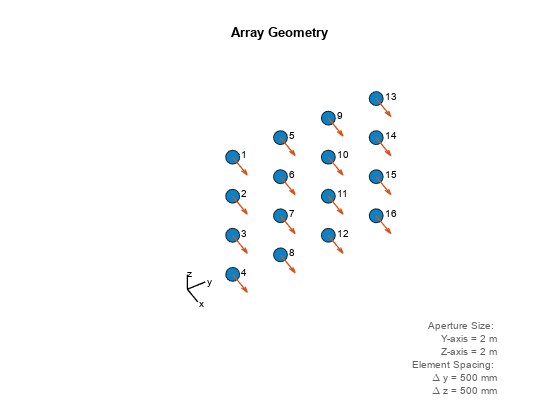
More About
The spacing between rows is the distance along the column axis direction between adjacent rows.

References
[1] Brookner, E., ed. Radar Technology. Lexington, MA: LexBook, 1996.
[2] Brookner, E., ed. Practical Phased Array Antenna Systems. Boston: Artech House, 1991.
[3] Mailloux, R. J. “Phased Array Theory and Technology,” Proceedings of the IEEE, Vol., 70, Number 3s, pp. 246–291.
[4] Mott, H. Antennas for Radar and Communications, A Polarimetric Approach. New York: John Wiley & Sons, 1992.
[5] Van Trees, H. Optimum Array Processing. New York: Wiley-Interscience, 2002.
Extended Capabilities
Version History
Introduced in R2011a