Factor Graph for SLAM

In the context of simultaneous localization and mapping (SLAM), a factor graph is a tool for estimating the most likely states of a robot and landmarks by integrating data from multiple sensors like lidar sensors, IMU sensors, GPS sensors, and cameras. This multisensor fusion improves the accuracy and robustness of state estimation.

Structurally, a factor graph is a bipartite graph, meaning it consists of two types of elements:

Nodes — The nodes represent the variables in the problem, such as the state of robot or vehicle and the position of landmarks in the environment. In conceptual graphs, nodes are shown as circles.
For a list of currently supported node types and their state format, see the Node Types section.
Factors — The factors represent the relationships or functions that define the dependencies between the nodes, typically using sensor measurements. In conceptual graphs, factors are shown as squares. For more information about factors, see the Factors section.
For a list of currently supported factors, see the List of Supported Factors section.

In Navigation Toolbox™, you can construct factor graphs using the factorGraph object.

Factor Graph Visualizations

You can visualize a factor graph spatially or conceptually. To show the differences, consider the factor graph of this code.

fg = factorGraph;
ids = generateNodeID(fg,3,"factorTwoPoseSE2");
f = factorTwoPoseSE2(ids,Measurement=relMeasure,Information=infoMatrix); % Measurements for factorTwoPoseSE2 factor are odometry sensor data
addFactor(fg,f);
nodeState(fg,unique(ids),initPoseGuess) % Set initial state guesses of pose nodes

Conceptual Visualization

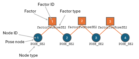
Conceptual visualization focuses on the relationship between nodes and factors in the graph and makes clear the bipartite quality of the factor graph. The position of nodes and factors in the graph does not provide any information about their current state. Nodes are represented as circles and factors are represented as squares. This figure shows the conceptual graph of the previously defined factor graph, fg.

Conceptual visualization of factor graph containing four SE(2) pose nodes connected by three factors.

Factors are defined as orange squares with their unique factor ID listed inside the factor and the factor type defined under the factor.

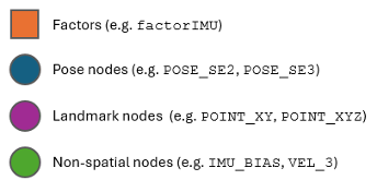
Nodes are defined as circles with their unique node ID listed inside the node and the node type defined under the node. This conceptual graph contains only pose nodes, but conceptual graphs can contain three types of nodes:

Pose nodes are blue, representing SE(2) or SE(3) pose nodes.
Landmark nodes are purple, representing xy- and xyz-points.
Nonspatial nodes are green, representing quantities that cannot be represented in physical space such as 3-D velocity and IMU gyroscope and accelerometer biases.

Legend for conceptual graph.

Spatial Visualization

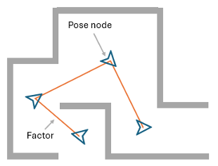
Spatial visualizations show the state of pose nodes and positions of landmarks with respect to each other. Nonspatial nodes, such as 3-D velocity and IMU gyroscope and accelerometer biases, do not appear in this visualization.

This figure shows the spatial visualization of the previously defined factor graph.

Spatial visualization of factor graph containing four SE(2) pose nodes connected by three factors.

You can use the show object function to plot a spatial visualization of a factor graph in MATLAB^®.

Probabilistic Model

Factor graphs provide a structured way to manage uncertainty by representing the joint probability distribution over robot states, landmark positions, and sensor measurements. By decomposing this distribution into simpler, local factors, factor graphs can represent the dependencies between these variables. This enables you to fuse different sensor measurements, such as IMU and GPS data, to improve the precision of state estimates through iterative optimization.

Factors

In a factor graph, factors act as edges connecting nodes, indicating the relationship between variables in the problem. Being a probabilistic model, the factor graph leverages these relationships to manage uncertainty and optimize solutions using data from multiple sources, like IMU and GPS sensors. This structure allows for efficient integration and processing of diverse sensor inputs to accurately estimate the variables of interest.

Factors can also be viewed as constraints on nodes, with the cost of a constraint indicating how well the node state aligns with real-world values. For example, in a robot with odometry, GPS, and IMU sensors, each sensor asserts observed information about the state of the pose node, and these constraints cumulatively make up a total cost. A low total cost suggests a high probability that the state estimate matches the actual state. Conversely, a high cost indicates a discrepancy between the state estimate and the actual state, requiring the optimizer to adjust the state estimate. This iterative process ensures the robot accurately determines its position and orientation.

Residuals

The cost associated with factors in the factor graph are derived from the residuals, which are the differences between the expected sensor readings, based on the current state estimate, and the actual sensor readings. The factor graph models the problem as a nonlinear least squares problem to minimize the residuals to refine the estimates of both robot and landmark states. Residuals are from errors in sensor measurements or inaccuracies in the motion model. The optimization process iteratively adjusts the state estimates to achieve the best possible fit to the data.

For example, factorTwoPoseSE2 factor calculates the residuals using this process using this information:

$p o s e_{i} = [\begin{matrix} x_{i} \\ y_{i} \\ θ_{i} \end{matrix}]$ , $p o s e_{j} = [\begin{matrix} x_{j} \\ y_{j} \\ θ_{j} \end{matrix}]$ — State estimates of the previous pose node i and current pose node j. Note that you can query the factor graph for the state estimate of nodes by using the nodeState object function.
$p o s e_{m} = [\begin{matrix} x_{m} \\ y_{m} \\ θ_{m} \end{matrix}]$ — Measured pose state. Note that measurement data for factors comes from sensors on the robot.
$I = [\begin{matrix} I_{x x} & I_{x y} & I_{x θ} \\ I_{x y} & I_{y y} & I_{y θ} \\ I_{θ x} & I_{θ y} & I_{θ θ} \end{matrix}]$ — Information matrix describing the precision and bias of the measured pose from the sensor.

Then the process for calculating the residuals for a factorTwoPoseSE2 factor is:

Calculate the residuals for the xy-position by creating an SO(2) rotation matrix from the prior orientation θ_i. Transpose this rotation matrix and use it to rotate the difference between the current pose and the prior pose, aligning it with the reference frame of the prior pose node. Finally, subtract the measured odometry pose from the result.

$[\begin{matrix} r e s_{x} \\ r e s_{y} \end{matrix}] = {[\begin{matrix} \cos θ_{i} & - \sin θ_{i} \\ \sin θ_{i} & \cos θ_{i} \end{matrix}]}^{T} \cdot ([\begin{matrix} x_{j} \\ y_{j} \end{matrix}] - [\begin{matrix} x_{i} \\ y_{i} \end{matrix}]) - [\begin{matrix} x_{m} \\ y_{m} \end{matrix}]$
Calculate the residuals for the orientation by subtracting the prior orientation and measured orientation from the current orientation.

$r e s_{θ} = θ_{j} - θ_{i} - θ_{m}$
Calculate the final residual values by taking the square root of the information matrix and multiplying it by the calculated pose residuals.

$r e s = \sqrt{I} \cdot [\begin{matrix} r e s_{x} \\ r e s_{y} \\ r e s_{θ} \end{matrix}]$

How to Use the `factorGraph` Object

This section shows how to start building a factor graph and provides tips and insights for ensuring well-constructed factor graphs.

Add Nodes and Factors

Constructing factor graphs relies on factor objects, which, when added to the graph, introduce both factors and any necessary nodes. A factor object connects to one or more nodes, depending on type of factor it represents. When you add a factor to the graph, if it specifies a node that does not exist, the graph automatically creates a node of the expected type to the factor graph. For example, in this case the graph is creating two new POSE_SE3 nodes with the node IDs 1 and 2 because neither node exists in the factor graph prior to the addition of the factor object.

fg = factorGraph;
f1 = factorTwoPoseSE3([1 2]);
% Add factor to factor graph and store the unique factor ID assigned by the factor graph.
fID = addFactor(fg,f1);

But if you add another factor to the same graph, you might be connecting to existing nodes. In this case, the factor connects to the existing node 2 and creates a new node with an ID of 3.

f2 = factorTwoPoseSE3([2 3]);
addFactor(fg,f2)

After adding factors to the factor graph, you must use the nodeState function to set an initial guess for the state of each node to provide more information to the optimizer. For example, this code shows how to set the initial states using the same factor graph.

initialGuessStates = [0 0 pi/2; 1 1 pi/4; 2 2 0] % [x y theta]
nodeState([1 2 3],initialGuessStates);

Setting initial guess states for nodes significantly improves the accuracy of the factor graph and helps prevent the optimization process from converging to local minima.

Match Node Types

When adding factors to a factor graph, make sure that you connect factors to node IDs of the correct node type.

The NodeID property of each factor object specifies and connects to these node types.:

Factor Object	Expected Node Types of Specified Node IDs
`factorGPS`	`["POSE_SE3"]`
`factorIMU`	`["POSE_SE3","VEL3","IMU_BIAS","POSE_SE3","VEL3","IMU_BIAS"]`
`factorCameraSE3AndPointXYZ`	`["POSE_SE3","POINT_XYZ"]` or `["POSE_SE3","POINT_XYZ","TRANSFORM_SE3"]`
`factorPoseSE2AndPointXY`	`["POSE_SE2","POINT_XY"]`
`factorPoseSE3AndPointXYZ`	`["POSE_SE3","POINT_XYZ"]`
`factorTwoPoseSE2`	`["POSE_SE2","POSE_SE2"]`
`factorTwoPoseSE3`	`["POSE_SE3","POSE_SE3"]`
`factorTwoPoseSIM3`	`["POSE_SE3","POSE_SE3_SCALE","POSE_SE3","POSE_SE3_SCALE"]`
`factorIMUBiasPrior`	`["IMU_BIAS"]`
`factorPoseSE3Prior`	`["POSE_SE3"]`
`factorVelocity3Prior`	`["VEL_3"]`

For example, factorPoseSE2AndPointXY([1 2]) creates a 2-D landmark factor connecting to node IDs 1 and 2. If you try to add that factor to a factor graph that already contains nodes with the IDs 1 and 2, the factor expects nodes 1 and 2 to be of types "POSE_SE2" and "POINT_XY", respectively.

You can also check the type of nodes in the factor graph by using the nodeType function.

fg = factorGraph;
f = factorTwoPoseSE2([1 2])
addFactor(fg,f);
typeID1 = nodeType(fg,1)

typeID1 = 
    "POSE_SE2"

Organize and Query Nodes

Node IDs enable you to perform many factor graph operations, so organizing these node IDs makes it easier to work with groups of nodes. You can organize nodes as you add them to a factor graph using the groupID argument of the addFactor. For more information about how to specify group IDs, see the groupID and the Add Nodes to Groups example.

Using the nodeIDs function, you can query node IDs in the factor graph in four ways:

All nodes at once — nodeIDs(fg); gets all nodes in the factor graph.
By node type — nodeIDs(fg,NodeType="POSE_SE2"); gets all nodes of type "POSE_SE2"
By factor type — nodeIDs(fg,FactorType="factorTwoPoseSE2") gets all nodes connected to factorTwoPoseSE2 factors.
By group ID — nodeIDs(fg,GroupID=1) gets all nodes in group 1.

For more information about how to get node IDs, see the Get Node IDs of Factor Graph example.

Optimize the Factor Graph

To optimize the factor graph, use the optimize object function. The optimize object function attempts to find a solution that minimizes the cost of the nonlinear least squares problem formulated by the factor graph. Note that the overall cost of the factor graph is the sum of the residuals of each factor, and the residual calculation varies according to the factor type.

Use one of two strategies to optimize your factor graph:

Global optimization — Optimize the entire factor graph each time you add new nodes and factors, or after you fully construct the graph. This strategy can yield the most accurate results compared to the sliding window workflow at the cost of a higher computation time.
Local optimization — Optimize the most recently added nodes and factors at each timestep. This optimization strategy is also known as sliding window optimization. This strategy is beneficial when dealing with large factor graphs because it minimizes the number of times that you need to reoptimize older parts of the factor graph. For an example of sliding window optimization, see Incrementally Optimize Factor Graph Using Sliding Window.

Note

Before optimizing a factor graph, set an initial state estimate for all nodes using the nodeState function.

You can also use the factorGraphSolverOptions object to specify and tune solver options. For more information about tuning the solver options, see the solnInfo output argument of the optimize object function.

Access Node States and Covariance

After optimization, you can access the current state of nodes using the nodeState function.

nID = 1;
states = nodeState(nID);

You can also get the node state covariance if you optimized with covariance calculation enabled. To enable covariance calculation, you must specify custom solver options using the factorGraphSolverOptions object, with the StateCovarianceType property set to the desired node types.

nID = 1;
cov = nodeCovariance(nID);

The factor graph optimization utilizes the Ceres Solver for node state covariance estimation. For more information about Ceres-Solver covariance estimation, see http://ceres-solver.org/nnls_covariance.html.

Note

Node state covariance estimation incurs higher computation costs and longer estimation times as the number of nodes being optimized increases.

Node Types

Each node in a factor graph is one of these types and has a corresponding state format.

POSE_SE2 — Pose in SE(2) state space in the form [x y theta]. x and y are the x- and y-positions, respectively, and theta is the orientation.
POSE_SE3 — Pose in SE(3) state space in the form [x y z qw qx qy qz]. x, y, and z are the x-, y-, and z-positions, respectively, and qw, qx, qy, and qz represent the orientation as a quaternion.
POSE_SE3_SCALE — Pose scale in SE(3) state space in the form of a variable s.
"TRANSFORM_SE3"— Sensor transform in SE(3) state space in the form [dx dy dz dqw dqx dqy dqz]. dx, dy, and dz are the change in position in x, y, and z respectively. dqw, dqx, dqy, and dqz are the change in quaternion rotation in w, x, y, and z, respectively.
VEL3 — 3-D velocity in the form [vx vy vz]. vx, vy, and vz are the x-, y-, and z-velocities, respectively.
POINT_XY — 2-D point in the form [x y]. x and y are the x- and y-positions, respectively.
POINT_XYZ — 3-D point in the form [x y z]. x, y, and z are the x-, y-, and z-positions, respectively.
IMU_BIAS — IMU gyroscope and accelerometer bias in the form [bias_gyro_x bias_gyro_y bias_gyro_z bias_accel_x bias_accel_y bias_accel_z], where:
- bias_gyro_x, bias_gyro_y, and bias_gyro_z are the x, y, and z IMU gyroscope biases, respectively.
- bias_accel_x, bias_accel_y, and bias_accel_z are the x, y, and z accelerometer biases, respectively.

List of Supported Factors

The factorGraph object supports the factors listed in the these sections by objective.

Relate Poses to Each Other

factorTwoPoseSE2 — Connect pairs of SE(2) pose nodes ("POSE_SE2") using relative pose measurements. You can calculate the relative pose using 2-D lidar scan registration using functions like matchScans.
factorTwoPoseSE3 — Connect pairs of SE(3) pose nodes ("POSE_SE3") using relative pose measurements. You can calculate the relative pose using 3-D lidar scan registration using functions like pcregistericp (Computer Vision Toolbox) and estrelpose (Computer Vision Toolbox).
factorTwoPoseSIM3 — Connect pairs of SIM(3) pose nodes using relative pose measurements. A SIM(3) pose node is represented using a combination of an SE(3) pose node ("POSE_SE3") and an SE(3) pose scale node ("POSE_SE3_SCALE"). You can use the estgeotform3d (Computer Vision Toolbox) function to calculate the relative pose measurement for this factor.

Relate Poses to Landmark Positions

factorCameraSE3AndPointXYZ — Connect the SE(3) pose node of a pinhole camera ("POSE_SE3") to 3-D landmark nodes ("Point_XYZ"), or the SE(3) pose node of a pinhole camera ("POSE_SE3"), 3-D landmark nodes ("Point_XYZ") , and an SE(3) sensor transform node ("TRANSFORM_SE3") using the 2-D image point measurements from the camera.
factorPoseSE2AndPointXY — Connect an SE(2) pose node ("POSE_SE2") to 2-D landmark nodes ("POINT_XY") using 2-D position measurements in the reference frame of the pose node.
factorPoseSE3AndPointXYZ — Connect an SE(3) pose node ("POSE_SE3") to 3-D landmark nodes ("POINT_XYZ") using 3-D position measurements in the reference frame of the pose node.

Relate Poses to Sensor Measurements

factorGPS — Connect an SE(3) pose node ("POSE_SE3") to a GPS measurement.
factorIMU — Connect two SE(3) pose nodes ("POSE_SE3"), two 3-D velocity nodes ("VEL3"), and two IMU bias nodes ("IMU_BIAS") using IMU measurements. These measurements consist of accelerometer and gyroscope data that capture changes in pose and velocity.

Relate Poses or Velocities to Prior-Known Measurements

If a pose, IMU bias, or velocity is a known quantity, add one of these prior factors to softly fix the node states, enabling slight variations only if doing so significantly reduces the overall cost:

factorIMUBiasPrior — Connect SE(3) pose nodes ("POSE_SE3"), 3-D velocity nodes ("VEL3"), and IMU bias nodes ("IMU_BIAS") to prior-known IMU measurements.
factorPoseSE3Prior — Connect SE(3) pose nodes ("POSE_SE3") to prior-known SE(3) pose measurements.
factorVelocity3Prior — Connect a 3-D velocity node ("VEL_3") to prior-known SE(3) velocity measurements.

For cases where certain node states must not vary at all during optimization, fix the nodes using the fixNode object function instead of adding a prior factor.