c2d
Convert model from continuous to discrete time
Description
sysd = c2d(sysc,Ts)sysc using zero-order hold on the inputs and a sample time of
Ts.
Examples
Discretize the following continuous-time transfer function:
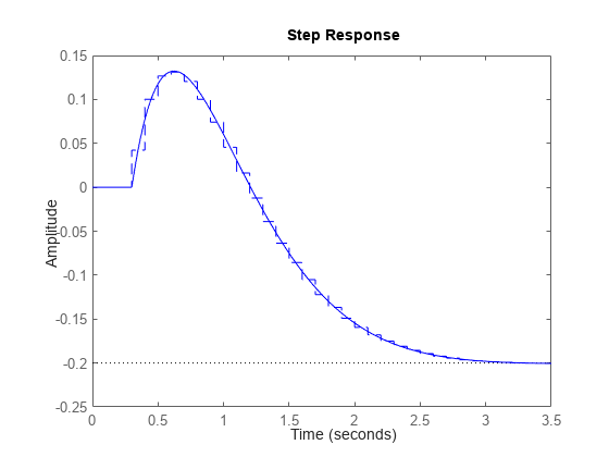
This system has an input delay of 0.3 s. Discretize the system using the triangle (first-order-hold) approximation with sample time Ts = 0.1 s.
H = tf([1 -1],[1 4 5],'InputDelay', 0.3);
Hd = c2d(H,0.1,'foh');
Compare the step responses of the continuous-time and discretized systems.
step(H,'-',Hd,'--')

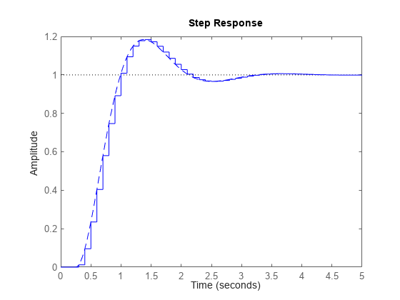
Discretize the following delayed transfer function using zero-order hold on the input, and a 10-Hz sampling rate.
h = tf(10,[1 3 10],'IODelay',0.25);
hd = c2d(h,0.1)
hd =
0.01187 z^2 + 0.06408 z + 0.009721
z^(-3) * ----------------------------------
z^2 - 1.655 z + 0.7408
Sample time: 0.1 seconds
Discrete-time transfer function.
Model Properties
In this example, the discretized model hd has a delay of three sampling periods. The discretization algorithm absorbs the residual half-period delay into the coefficients of hd.
Compare the step responses of the continuous-time and discretized models.
step(h,'--',hd,'-')

Since R2024a
Create a continuous-time state-space model with two states and an input delay.
sys = ss(tf([1,2],[1,4,2]));
sys.InputDelay = 2.7
sys =

  A =
       x1  x2
   x1  -4  -2
   x2   1   0

  B =
       u1
   x1   2
   x2   0

  C =
        x1   x2
   y1  0.5    1

  D =
       u1
   y1   0

  Input delays (seconds): 2.7

Continuous-time state-space model.
Model Properties
Discretize the model using the Tustin discretization method and a Thiran filter to model fractional delays. The sample time Ts = 1 second.
opt = c2dOptions('Method','tustin','ThiranOrder',3);
sysd1 = c2d(sys,1,opt)
sysd1 =

  A =
            x1       x2
   x1  -0.4286  -0.5714
   x2   0.2857   0.7143

  B =
           u1
   x1  0.5714
   x2  0.2857

  C =
           x1      x2
   y1  0.2857  0.7143

  D =
           u1
   y1  0.2857

  (values computed with all internal delays set to zero)

  Internal delays (sampling periods): 1  1  1

Sample time: 1 seconds
Discrete-time state-space model.
Model Properties
By default, the function models extra delays as internal delays in the discretized model. To model extra delays as states in the discretized model, set the DelayModeling option of c2dOptions to 'state'.
opt2 = c2dOptions('Method','tustin','ThiranOrder',3,'DelayModeling','state');
sysd2 = c2d(sys,1,opt2)
sysd2 =

  A =
              x1         x2         x3         x4         x5
   x1    -0.4286    -0.5714   -0.00265    0.06954      2.286
   x2     0.2857     0.7143  -0.001325    0.03477      1.143
   x3          0          0    -0.2432     0.1449    -0.1153
   x4          0          0       0.25          0          0
   x5          0          0          0      0.125          0

  B =
             u1
   x1  0.002058
   x2  0.001029
   x3         8
   x4         0
   x5         0

  C =
              x1         x2         x3         x4         x5
   y1     0.2857     0.7143  -0.001325    0.03477      1.143

  D =
             u1
   y1  0.001029

Sample time: 1 seconds
Discrete-time state-space model.
Model Properties
The discretized model now contains three additional states x3, x4, and x5 corresponding to a third-order Thiran filter. Since the time delay divided by the sample time is 2.7, the third-order Thiran filter ('ThiranOrder' = 3) can approximate the entire time delay.
Estimate a continuous-time transfer function, and discretize it.
load iddata1
sys1c = tfest(z1,2);
sys1d = c2d(sys1c,0.1,'zoh');
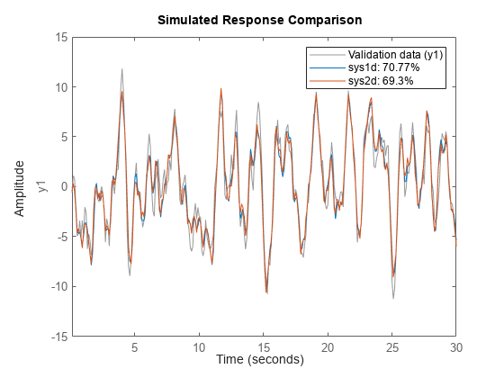
Estimate a second order discrete-time transfer function.
sys2d = tfest(z1,2,'Ts',0.1);Compare the response of the discretized continuous-time transfer function model, sys1d, and the directly estimated discrete-time model, sys2d.
compare(z1,sys1d,sys2d)

The two systems are almost identical.
Discretize an identified state-space model to build a one-step ahead predictor of its response.
Create a continuous-time identified state-space model using estimation data.
load iddata2
sysc = ssest(z2,4);
Predict the 1-step ahead predicted response of sysc.
predict(sysc,z2)

Discretize the model.
sysd = c2d(sysc,0.1,'zoh');Build a predictor model from the discretized model, sysd.
[A,B,C,D,K] = idssdata(sysd);
Predictor = ss(A-K*C,[K B-K*D],C,[0 D],0.1);
Predictor is a two-input model which uses the measured output and input signals ([z1.y z1.u]) to compute the 1-step predicted response of sysc.
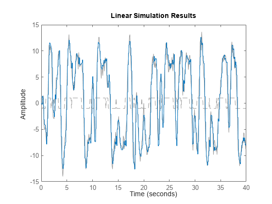
Simulate the predictor model to get the same response as the predict command.
lsim(Predictor,[z2.y,z2.u])

The simulation of the predictor model gives the same response as predict(sysc,z2).
Input Arguments
Continuous-time model, specified as a dynamic system model such as idtf, idss, or idpoly.
sysc cannot be a frequency response data model.
sysc can be a SISO or MIMO system, except that the
'matched' discretization method supports SISO systems
only.
sysc can have input/output or internal time delays;
however, the 'matched', 'impulse', and
'least-squares' methods do not support state-space
models with internal time delays.
The following identified linear systems cannot be discretized directly:
idgreymodels whoseFunctionTypeis'c'. Convert toidssmodel first.idprocmodels. Convert toidtforidpolymodel first.
Sample time, specified as a positive scalar that represents the sampling
period of the resulting discrete-time system. Ts is in
TimeUnit, which is the
sysc.TimeUnit property.
Discretization method, specified as one of the following values:
'zoh'— Zero-order hold (default). Assumes the control inputs are piecewise constant over the sample timeTs.'foh'— Triangle approximation (modified first-order hold). Assumes the control inputs are piecewise linear over the sample timeTs.'impulse'— Impulse invariant discretization'tustin'— Bilinear (Tustin) method. To specify this method with frequency prewarping (formerly known as the'prewarp'method), use thePrewarpFrequencyoption ofc2dOptions.'matched'— Zero-pole matching method'least-squares'— Least-squares method'damped'— Damped Tustin approximation based on theTRBDF2formula forsparssmodels only.
For information about the algorithms for each conversion method, see Continuous-Discrete Conversion Methods.
Discretization options, specified as a c2dOptions object. For
example, specify the prewarp frequency, order of the Thiran filter or
discretization method as an option.
Output Arguments
Discrete-time model, returned as a dynamic system model of the same type
as the input system sysc.
When sysc is an identified (IDLTI) model,
sysd:
Includes both measured and noise components of
sysc. The innovations variance λ of the continuous-time identified modelsysc, stored in itsNoiseVarianceproperty, is interpreted as the intensity of the spectral density of the noise spectrum. The noise variance insysdis thus λ/Ts.Does not include the estimated parameter covariance of
sysc. If you want to translate the covariance while discretizing the model, usetranslatecov.
Mapping of continuous-time initial conditions x0 and u0 of the state-space model sysc to the
discrete-time initial state vector x[0], returned as a matrix. The mapping of initial conditions
to the initial state vector is as follows:
For state-space models with time delays, when
DelayModeling = "state", c2d
pads the matrix G with zeros to account for additional
states introduced by discretizing those delays.
For state-space models with internal delays,
c2d returns an additional columns for
w[0].
The mapping of the discrete states is given by:
The matrix G is useful to map continuous-time initial
conditions to equivalent discrete-time initial conditions. Note that this
expression depends on the input u delayed by the discrete
input delays Nu.
See Continuous-Discrete Conversion Methods for a discussion of modeling time delays in discretized systems.
Version History
Introduced before R2006aThe output argument G now has extra columns corresponding to
w[0] initial conditions for models with internal
delays.
The c2d command no longer adds extra states when modeling
extra delays. By default, c2d now uses internal delays and
returns the discretized model with the same number of states. This results in a more
predictable behavior and simplifies initial state mapping from continuous to
discrete time.
To revert to the old behavior before R2024a, create an option set using
c2dOptions and set DelayModeling to
"state".
You can now discretize mechss models using the bilinear Tustin
approximation method. For mechss models, the
'tustin' method computes the second-order form of the Tustin
discretization. This is equivalent to applying Tustin to the first-order
sparss equivalent of the mechss model.
You can now use c2d to discretize models with offsets such as
gridded linear parameter varying models.
Additionally, c2dOptions provides two new
options
DelayModeling— Specify whether to model extra delays as internal delays (default) or additional states.Consistency— Enforce state and delay consistency in state-space arrays. This option is helpful when discretizing gridded LPV or LTV models.
See Also
c2dOptions | d2c | d2d | thiran (Control System Toolbox) | translatecov
MATLAB Command
You clicked a link that corresponds to this MATLAB command:
Run the command by entering it in the MATLAB Command Window. Web browsers do not support MATLAB commands.
Select a Web Site
Choose a web site to get translated content where available and see local events and offers. Based on your location, we recommend that you select: .
You can also select a web site from the following list
How to Get Best Site Performance
Select the China site (in Chinese or English) for best site performance. Other MathWorks country sites are not optimized for visits from your location.
Americas
- América Latina (Español)
- Canada (English)
- United States (English)
Europe
- Belgium (English)
- Denmark (English)
- Deutschland (Deutsch)
- España (Español)
- Finland (English)
- France (Français)
- Ireland (English)
- Italia (Italiano)
- Luxembourg (English)
- Netherlands (English)
- Norway (English)
- Österreich (Deutsch)
- Portugal (English)
- Sweden (English)
- Switzerland
- United Kingdom (English)