Configure Time Scope MATLAB Object
When you use the timescope object in MATLAB®, you can configure many settings and tools from the window. These sections
show how to use the Time Scope interface and the available tools.
Signal Display
These figures highlight the important aspects of the Time Scope window in MATLAB.
Scope Tab
Measurements Tab
Min X-Axis — Time scope sets the minimum x-axis limit using the value of the
TimeDisplayOffsetproperty. To change the Time Offset from the Time Scope window, click Settings ( ) on the Scope tab. Under
Data and Axes, set the Time
Offset.
) on the Scope tab. Under
Data and Axes, set the Time
Offset.Max X-Axis — Time scope sets the maximum x-axis limit by summing the value of the Time Offset property with the span of the x-axis values. If Time Span is set to
Auto, the span of x-axis is10/SampleRate.The values on the x-axis of the scope display remain the same throughout the simulation.
Status — Provides the current status of the plot. The status can be:
Processing— Occurs after you run the object and before you run thereleasefunction.Stopped— Occurs after you create the scope object and before you first call the object. This status also occurs after you callrelease.
Title, Y-Label — You can customize the title and the y-axis label from Settings or by using the
TitleandYLabelproperties.Toolstrip
Scope tab — Customize and share the time scope. For example, showing and hiding the legend.
Measurements tab — Turn on and control different measurement tools.
Use the pin button
 to keep the toolstrip showing or the
arrow button
to keep the toolstrip showing or the
arrow button  to hide the toolstrip.
Multiple Signal Names and Colors
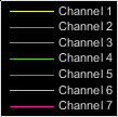
By default, if the input signal has multiple channels, the scope uses an index number
to identify each channel of that signal. For example, the legend for a two-channel
signal will display the default names Channel 1, Channel
2. To show the legend, on the Scope tab, click
Settings (![]() ). Under Display and Labels, select
Show Legend. If there are a total of seven input channels, the
legend displayed is:
). Under Display and Labels, select
Show Legend. If there are a total of seven input channels, the
legend displayed is:
By default, the scope has a black axes background and chooses line colors for each channel in a manner similar to the Simulink® Scope (Simulink) block. When the scope axes background is black, it assigns each channel of each input signal a line color in the order shown in the legend. If there are more than seven channels, then the scope repeats this order to assign line colors to the remaining channels. When the axes background is not black, the signals are colored in this order:

To choose line colors or background colors, on the Scope tab click Settings. Use the Axes color pallet to change the background of the plot. Click Line to choose a line to change, and the Color drop-down to change the line color of the selected line.
Configure Scope Settings
On the Scope tab, the Settings section allows you to modify the scope.
The Legend button turns the legend on or off. When you show the legend, you can control which signals are shown. If you click a signal name in the legend, the signal is hidden from the plot and shown in gray on the legend. To redisplay the signal, click on the signal name again. This button corresponds to the
ShowLegendproperty in the object.The Settings button opens the settings window which allows you to customize the data, axes, display settings, labels, and color settings.
The Display Grid button enables you to select the display layout of the scope.
Use timescope Measurements and Triggers
All measurements are made for a specified channel. By default, measurements are applied to the first channel. To change which channel is being measured, use the Select Channel drop-down on the Measurements tab.
Data Cursors
Use the Data Cursors button to display screen and waveform cursors. Each cursor tracks a vertical line along the signal. The difference between x- and y-values of the signal at the two cursors is displayed in the box between the cursors.
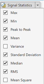
Signal Statistics
Use the Signal Statistics button to display statistics
about the selected signal at the bottom of the time scope window. You can hide or
show the Statistics panel using the arrow button ![]() at the bottom right of the panel.
at the bottom right of the panel.
Max — Maximum value within the displayed portion of the input signal.
Min — Minimum value within the displayed portion of the input signal.
Peak to Peak — Difference between the maximum and minimum values within the displayed portion of the input signal.
Mean — Average or mean of all the values within the displayed portion of the input signal.
Variance — Variance of the values within the displayed portion of the input signal.
Standard Deviation — Standard deviation of the values within the displayed portion of the input signal.
Median — Median value within the displayed portion of the input signal.
RMS — Root mean square of the input signal.
Mean Square — Mean square of the values within the displayed portion of the input signal.
To customize which statistics to show and compute, use the Signal Statistics list.
Peak Finder
Use the Peak Finder button to display peak values
for the selected signal. Peaks are defined as a local maximum where lower values are
present on both sides of a peak. End points are not considered peaks. For more
information on the algorithms used, see the findpeaks (Signal Processing Toolbox) function.
When you turn on the peak finder measurements, an arrow appears on the plot at
each maxima and a Peaks panel appears at the bottom of the
timescope window showing the x and
y values at each peak.
You can customize several peak finder settings:
Label Peaks — Show labels (P1, P2, …) above the arrows on the plot.
Num Peaks — The number of peaks to show. Must be a scalar integer from 1 through 99.
Min Height — The minimum height difference between a peak and its neighboring samples.
Min Distance — The minimum number of samples between adjacent peaks.
Threshold — The level above which peaks are detected.
Bilevel Measurements
With bilevel measurements, you can measure transitions, aberrations, and cycles.
Bilevel Settings. When using bilevel measurements, you can set these properties:
Auto State Level — When this check box is selected, the Bilevel measurements panel detects the high- and low-state levels of a bilevel waveform. When this check box is cleared, you can enter in values for the high- and low-state levels manually.
High — Manually specify the value that denotes a positive polarity or high-state level.

Low — Manually specify the value that denotes a negative polarity or low-state level.
State Level Tol. (%) — Tolerance levels within which the initial and final levels of each transition must lie to be within their respective state levels. This value is expressed as a percentage of the difference between the high- and low-state levels.
Upper Ref. Level (%) — Used to compute the end of the rise-time measurement or the start of the fall-time measurement. This value is expressed as a percentage of the difference between the high- and low-state levels.
Mid Ref. Level (%) — Used to determine when a transition occurs. This value is expressed as a percentage of the difference between the high- and low-state levels. In the following figure, the mid-reference level is shown as a horizontal line, and its corresponding mid-reference level instant is shown as a vertical line.

Lower Ref. Level (%) — Used to compute the end of the fall-time measurement or the start of the rise-time measurement. This value is expressed as a percentage of the difference between the high- and low-state levels.
Settle Seek (s) — The duration after the mid-reference level instant when each transition occurs is used for computing a valid settling time. Settling time is displayed in the Aberrations pane.
Transitions. Select Transitions to display calculated measurements associated with the input signal changing between its two possible state level values, high and low. The measurements are displayed in the Transitions pane at the bottom of the scope window.
The + Edges row measures rising edges or a positive-going transition. A rising edge in a bilevel waveform is a transition from the low-state level to the high-state level with a slope value greater than zero.
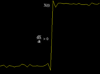
The - Edges row measures falling edges or a negative-going transition. A falling edge in a bilevel waveform is a transition from the high-state level to the low-state level with a slope value less than zero.
The Transition measurements assume that the amplitude of the input signal is in units of volts. For the transition measurements to be valid, you must convert all input signals to volts.
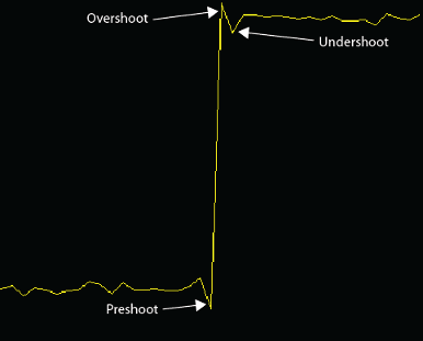
Aberrations. Select Aberrations to display calculated measurements involving the distortion and damping of the input signal such as preshoot, overshoot, and undershoot. Overshoot and undershoot, respectively, refer to the amount that a signal exceeds and falls below its final steady-state value. Preshoot refers to the amount before a transition that a signal varies from its initial steady-state value. The measurements are displayed in the Transitions pane at the bottom of the scope window.
This figure shows preshoot, overshoot, and undershoot for a rising-edge transition.
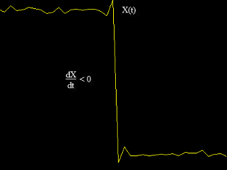
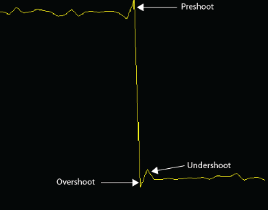
The next figure shows preshoot, overshoot, and undershoot for a falling-edge transition.
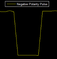
Cycles. Select Cycles calculates repetitions or trends in the displayed portion of the input signal. The measurements are displayed in the Cycles pane at the bottom of the scope window in two rows: + Pulses for the positive-polarity pulses and - Pulses for the negative-polarity pulses.
Period — Average duration between adjacent edges of identical polarity within the displayed portion of the input signal. To calculate period, the
timescopetakes the difference between the mid-reference level instants of the initial transition of each pulse and the next identical-polarity transition. These mid-reference level instants for a positive-polarity pulse appear as red dots in the following figure.
Frequency — Reciprocal of the average period, measured in hertz.
Count — Number of positive- or negative-polarity pulses counted.
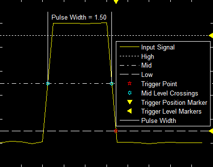
Width — Average duration between rising and falling edges of each pulse within the displayed portion of the input signal.
Duty Cycle — Average ratio of pulse width to pulse period for each pulse within the displayed portion of the input signal.
Triggers
Define a trigger event to identify the simulation time of specified input signal characteristics. You can use trigger events to stabilize periodic signals such as a sine wave or capture non-periodic signals such as a pulse that occurs intermittently.
To define a trigger:
On the Trigger tab of the scope window, select the channel you want to trigger.
Specify when the display updates by selecting a triggering Mode.
Auto — Display data from the last trigger event. If no event occurs after one time span, display the last available data.
Normal — Display data from the last trigger event. If no event occurs, the display remains blank.
Once — Display data from the last trigger event and freeze the display. If no event occurs, the display remains blank. Click the Rearm Trigger button to look for the next trigger event.
Select a triggering type, polarity, and any other properties. See the Trigger Properties table.
Click Enable Trigger.
You can set the trigger position to specify the position of the time pointer along the y-axis. You can also drag the time pointer to the left or right to adjust its position.
Trigger Properties
| Trigger Type | Trigger Parameters |
|---|---|
| Polarity — Select the polarity for an edge-triggered signal.
Level — Enter a threshold value for an edge-triggered signal. Auto level is 50% Hysteresis — Enter a value for an edge-triggered signal. See Hysteresis of Trigger Signals Delay (s) — Offset the trigger by a fixed delay in seconds. Holdoff (s) — Set the minimum possible time between triggers. Position (%) — Set horizontal position of the trigger on the screen. |
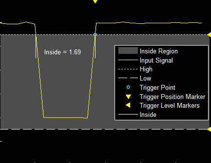
| Polarity — Select the polarity for a pulse width-triggered signal.
Note A glitch-trigger is a special type of a pulse width-trigger. A glitch-trigger occurs for a pulse or spike whose duration is less than a specified amount. You can implement a glitch-trigger by using a pulse-width-trigger and setting the Max Width parameter to a small value. High — Enter a high value for a pulse-width-triggered signal. Auto level is 90%. Low — Enter a low value for a pulse-width-triggered signal. Auto level is 10%. Min Width (s) — Enter the minimum pulse width for a pulse-width-triggered signal. Pulse width is measured between the first and second crossings of the middle threshold. Max Width (s) — Enter the maximum pulse width for a pulse-width-triggered signal. Delay (s) — Offset the trigger by a fixed delay in seconds. Holdoff (s) — Set the minimum possible time between triggers. Position (%) — Set horizontal position of the trigger on the screen. |
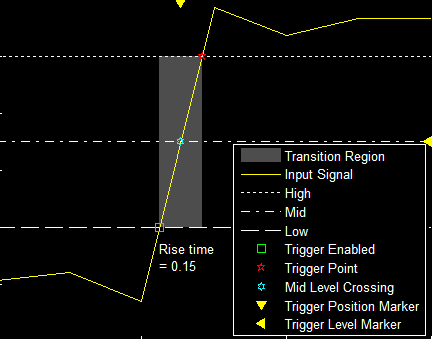
| Polarity — Select the polarity for a transition-triggered signal.
High — Enter a high value for a transition-triggered signal. Auto level is 90%. Low — Enter a low value for a transition-triggered signal. Auto level is 10%. Min Time (s) — Enter a minimum time duration for a transition-triggered signal. Max Time (s) — Enter a maximum time duration for a transition-triggered signal. Delay (s) — Offset the trigger by a fixed delay in seconds. Holdoff (s) — Set the minimum possible time between triggers. Position (%) — Set horizontal position of the trigger on the screen. |
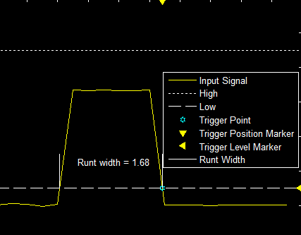
| Polarity — Select the polarity for a runt-triggered signal.
High — Enter a high value for a runt-triggered signal. Auto level is 90%. Low — Enter a low value for a runt-triggered signal. Auto level is 10%. Min Width (s) — Enter a minimum width for a runt-triggered signal. Pulse width is measured between the first and second crossing of a threshold. Max Width (s) — Enter a maximum pulse width for a runt-triggered signal. Delay (s) — Offset the trigger by a fixed delay in seconds. Holdoff (s) — Set the minimum possible time between triggers. Position (%) — Set horizontal position of the trigger on the screen. |
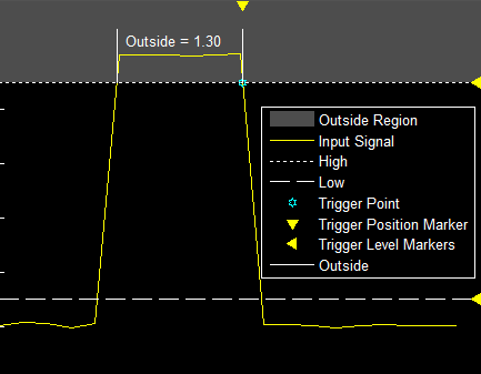
| Polarity — Select the region for a window-triggered signal.
High — Enter a high value for a window-triggered signal. Auto level is 90%. Low — Enter a low value for a window-trigger signal. Auto level is 10%. Min Time (s) — Enter the minimum time duration for a window-triggered signal. Max Time (s) — Enter the maximum time duration for a window-triggered signal. Delay (s) — Offset the trigger by a fixed delay in seconds. Holdoff (s) — Set the minimum possible time between triggers. Position (%) — Set horizontal position of the trigger on the screen. |
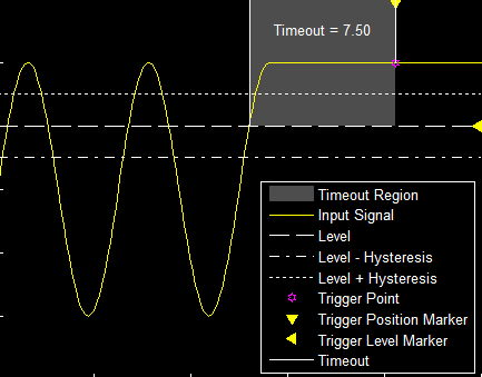
| Polarity — Select the polarity for a timeout-triggered signal.
Level — Enter a threshold value for a timeout-triggered signal. Hysteresis — Enter a value for a timeout-triggered signal. See Hysteresis of Trigger Signals. Timeout (s) — Enter a time duration for a timeout-triggered signal. Alternatively, a trigger event can occur when the signal stays within the boundaries defined by the hysteresis for 7.50 seconds after the signal crosses the threshold.
Delay (s) — Offset the trigger by a fixed delay in seconds. Holdoff (s) — Set the minimum possible time between triggers. Position (%) — Set horizontal position of the trigger on the screen. |
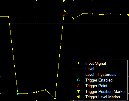
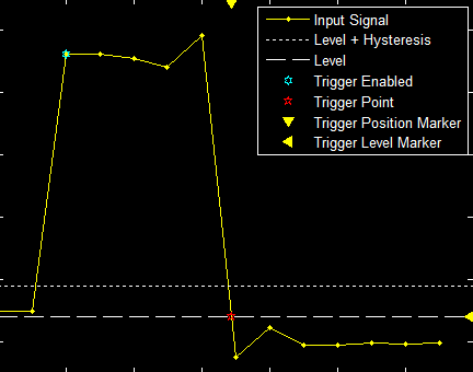

Hysteresis of Trigger Signals
Hysteresis — Specify the hysteresis or noise-reject value.
This parameter is visible when you set Type to
Edge or Timeout. If the
signal jitters inside this range and briefly crosses the trigger level, the scope
does not register an event. In the case of an edge trigger with rising polarity, the
scope ignores the times that a signal crosses the trigger level within the
hysteresis region.

You can reduce the hysteresis region size by decreasing the hysteresis value. In this example, if you set the hysteresis value to 0.07, the scope also considers the second rising edge to be a trigger event.

Share or Save the Time Scope
If you want to save the time scope for future use or share it with others, use the buttons in the Share section of the Scope tab.
Generate Script — Generate a script to re-create your time scope with the same settings. An editor window opens with the code required to re-create your
timescopeobject.
Copy to Clipboard — Copy the display to your clipboard. You can paste the image in another program to save or share it.
Preserve Colors –– Preserve colors while copying to the clipboard.
Print — Opens a print dialog box from which you can print out the plot image.
Scale Axes
To scale the plot axes, you can use the mouse to pan around the axes and the scroll button on your mouse to zoom in and out of the plot. Additionally, you can use the buttons that appear when you hover over the plot window.
 — Maximize the axes, hide all labels and
inset the axes values.
— Maximize the axes, hide all labels and
inset the axes values.
 — Zoom in and out of the plot.
 — Pan the plot.
 — Autoscale the x and
y axes of the current display to fit the shown
data.
— Autoscale the x and
y axes of the current display to fit the shown
data.