Returns with Negative Prices
Once considered a mathematical impossibility, negative prices have become an established aspect of many financial markets. Negative prices arise in situations where investors determine that holding an asset entails more risk than the current value of the asset. For example, energy futures see negative prices because of costs associated with overproduction and limited storage capacity. In a different setting, central banks impose negative interest rates when national economies become deflationary, and the pricing of interest rate derivatives, traditionally based on positivity, have to be rethought (see Work with Negative Interest Rates Using Functions (Financial Instruments Toolbox)). A negative price encourages the buyer to take something from the seller, and the seller pays a fee for the service of divesting.
MathWorks® Computational Finance products support several functions for converting between price series p(t) and return series r(t). Price positivity is not a requirement. The returns computed from input negative prices can be unexpected, but they have mathematical meaning that can help you to understand price movements.
Negative Price Conversion
Financial Toolbox™ functions ret2tick and tick2ret support converting between price series
p(t) and return series
r(t).
For simple returns (default), the functions implement the formulas
For continuous returns, the functions implement the formulas
The functions price2ret (Econometrics Toolbox) and ret2price (Econometrics Toolbox) implement the same formulas, but they divide by
Δt in the return formulas and they multiply by Δt in
the price formulas. A positive factor of Δt (enforced by required
monotonic observation times) does not affect the behavior of the functions. Econometrics Toolbox™ calls simple returns periodic, and
continuous returns are the default. Otherwise, the functionality between the set of
functions is identical. This example concentrates on the Financial Toolbox functions.
In the simple return formula, rs(t) is the percentage change (PC) in ps(t − 1) over the interval [t − 1,t]
For positive prices, the range of PC is (−1,∞), that is, anything from a 100% loss (ps: ps(t − 1) → 0) to unlimited gain. The recursion in the second equation gives the subsequent prices; ps(t) is computed from ps(t − 1) by adding a percentage of ps(t − 1).
Furthermore, you can aggregate simple returns through time using the formula
where the left-hand side represents the simple return over the entire interval [0,T].
Continuous returns add 1 to PC to move the range to (0,∞), the domain of the real logarithm. Continuous returns have the time aggregation property
This transformation ensures additivity of compound returns.
If negative prices are allowed, the range of simple returns PC expands to (−∞,∞), that is, anything from unlimited loss to unlimited gain. In the formula for continuous returns, logarithms of negative numbers are unavoidable. The logarithm of a negative number is not a mathematical problem because the complex logarithm (the MATLAB® default) interprets negative numbers as complex numbers with phase angle ±π, so that, for example,
If x < 0, log(x) = log(|x|) ± iπ. The log of a negative number has an imaginary part of ±π. The log of 0 is undefined because the range of the exponential eiθ is positive. Therefore, zero prices (that is, free exchanges) are unsupported.
Analysis of Negative Price Returns
To illustrate negative price inputs, consider the following price series and its simple returns.
p = [3; 1; -2; -1; 1]
p =

     3
     1
    -2
    -1
     1
rs = tick2ret(p)
rs =

   -0.6667
   -3.0000
   -0.5000
   -2.0000
This table summarizes the recursions.
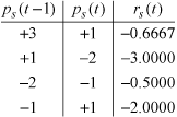
The returns have the correct size (66%, 300%, 50%, 200%), but do they have the correct sign? If you interpret negative returns as losses, as with the positive price series, the signs seem wrong—the last two returns should be gains (that is, if you interpret less negative to be a gain). However, if you interpret the negative returns by the formula
which requires the signs, the last two negative percentage changes multiply negative prices ps(t − 1), which produces positive additions to ps(t − 1). Briefly, a negative return on a negative price produces a positive price movement. The returns are correct.
The round trip produced by ret2tick returns
the original price series.
ps = ret2tick(rs,StartPrice=3)
ps =

     3
     1
    -2
    -1
     1
Also, the following computations shows that time aggregation holds.
p(5)/p(1) - 1
ans =

   -0.6667
prod(rs + 1) - 1
ans =

   -0.6667
For continuous returns, negative price ratios pc(t)/pc(t − 1) are interpreted as complex numbers with phase angles ±π, and the complex logarithm is invoked.
rc = tick2ret(p,Method="continuous")
rc =

  -1.0986 + 0.0000i
   0.6931 + 3.1416i
  -0.6931 + 0.0000i
   0.0000 - 3.1416i
This table summarizes the recursions.
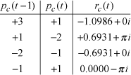
The real part shows the trend in the absolute price series. When |pc(t − 1)| < |pc(t)|, that is, when prices move away from zero, rc(t) has a positive real part. When |pc(t − 1)| > |pc(t)|, that is, when prices move toward zero, rc(t) has a negative real part. When |pc(t − 1)| = |pc(t)|, that is, when the absolute size of the prices is unchanged, rc(t) has a zero real part. For positive price series, where the absolute series is the same as the series itself, the real part has its usual meaning.
The imaginary part shows changes of sign in the price series. When pc(t − 1) > 0 and pc(t) < 0, that is, when prices move from investments to divestments, rc(t) has a positive imaginary part (+π). When pc(t − 1) < 0 and pc(t) > 0, that is, when prices move from divestments to investments, rc(t) has a negative imaginary part (−π). When the sign of the prices is unchanged, rc(t) has a zero imaginary part. For positive price series, changes of sign are irrelevant, and the imaginary part conveys no information (0).
Visualization of Complex Returns
Complex continuous returns contain a lot of information. Visualizing the information can help you to interpret the complex returns. The following code plots the real and imaginary parts of the logarithm on either side of zero.
p = -5:0.01:5;
hold on
plot(p,real(log(p)),"b")
plot(p,imag(log(p)),"r")
xticks(-5:5)
xlabel("Price (p)")
ylabel("Ordinate")
legend(["real(log(p))" "imag(log(p))"],AutoUpdate=false)
grid minor
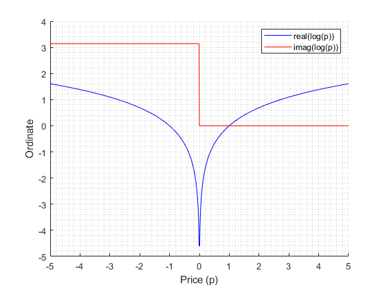
Due to the following identity
you can read the real part of a continuous return as a difference in ordinates on the blue graph, and you can read the imaginary part as a difference in ordinates on the red graph. Absolute price movements toward zero result in a negative real part and absolute price movements away from zero result in a positive real part. Likewise, changes of sign result in a jump of ±π in the imaginary part, with the sign change depending on the direction of the move.
For example, the plot below superimposes the real and imaginary parts of the logarithm at prices p = −4 and p = 2, with lines to help visualize their differences.
p = [-4; 2];
plot(p,real(log(p)),"bo-",MarkerFaceColor="b")
plot(p,imag(log(p)),"ro-",MarkerFaceColor="r")
hold off
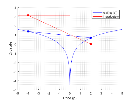
If pc(t − 1) = −4 and pc(t) = 2, the real part of log(pc(t)) − log(pc(t − 1)) is negative (line slopes down), corresponding to a decrease in absolute price. The imaginary part is 0 – π = −π, corresponding to a change of sign from negative to positive. If the direction of the price movement is reversed, so that pc(t − 1) = 2 and pc(t) = −4, the positive difference in the real part corresponds to an increase in absolute price, and the positive difference in the imaginary part corresponds to a change of sign from positive to negative.
If you convert the continuous returns rc(t) = log(pc(t)/pc(t − 1) ) to simple returns rs = (ps(t)/ps(t − 1) − 1) by the following computation, the result is the same simple returns series as before.
rs = exp(rc) - 1
rs =

  -0.6667 + 0.0000i
  -3.0000 + 0.0000i
  -0.5000 + 0.0000i
  -2.0000 - 0.0000i
pc = ret2tick(rc,Method="continuous",StartPrice=3)pc = 3.0000 + 0.0000i 1.0000 + 0.0000i -2.0000 + 0.0000i -1.0000 + 0.0000i 1.0000 + 0.0000i
Conclusion
Complex continuous returns are a necessary intermediary when considering logarithms of
negative price ratios. tick2ret computes a continuous complex
extension of the function on the positive real axis. The logarithm maintains the additivity
property, used when computing multiperiod returns.
Because of the extensible logarithm implemented in MATLAB, current implementations of Computational Finance tools that accept prices and returns behave logically with negative prices. The interpretation of complex-valued results can be unfamiliar at first, but as shown, the results are meaningful and explicable.
See Also
Topics
- Work with Negative Interest Rates Using Functions (Financial Instruments Toolbox)