price2ret

Convert prices to returns

Syntax

[Returns,intervals] = price2ret(Prices)

ReturnTbl = price2ret(PriceTbl)

[___] = price2ret(___,Name=Value)

Description

[Returns,intervals] = price2ret(Prices) returns the matrix of numVars continuously compounded return series Returns, and corresponding time intervals intervals, from the matrix of numVars price series Prices.

ReturnTbl = price2ret(PriceTbl) returns the table or timetable of continuously compounded return series ReturnTbl of each variable in the table or timetable of price series PriceTbl. To select different variables in Tbl from which to compute returns, use the DataVariables name-value argument.

[___] = price2ret(___,Name=Value) specifies options using one or more name-value arguments in addition to any of the input argument combinations in previous syntaxes. price2ret returns the output argument combination for the corresponding input arguments. For example, price2ret(Tbl,Method="periodic",DataVariables=1:5) computes the simple periodic returns of the first five variables in the input table Tbl.

Examples

Compute Return Series from Price Series in Vector of Data

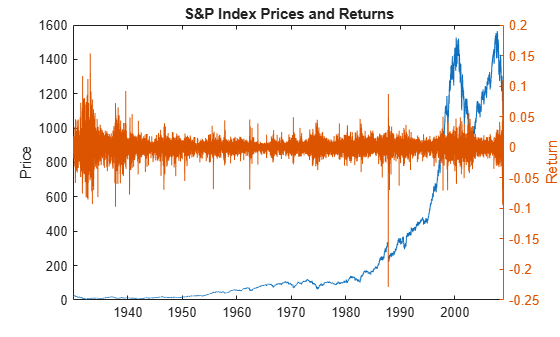
Load the Schwert Stock data st Data_SchwertStock.mat, which contains daily prices of the S&P index from 1930 through 2008, among other variables (enter Description for more details).

load Data_SchwertStock
numObs = height(DataTableDly)

numObs = 20838

dates = datetime(datesDly,ConvertFrom="datenum");

Convert the S&P price series to returns.

prices = DataTableDly.SP;
returns = price2ret(prices);

returns is a 20837-by-1 vector of daily S&P returns compounded continuously.

r9 = returns(9)

r9 = 0.0033

p9_10 = [prices(9) prices(10)]

p9_10 = 1×2

   21.4500   21.5200

returns(9) = 0.0033 is the daily return of the prices in the interval [21.45, 21.52].

plot(dates,DataTableDly.SP)
ylabel("Price")
yyaxis right
plot(dates(1:end-1),returns)
ylabel("Return")
title("S&P Index Prices and Returns")

Compute Simple Periodic Return Series from Table of Price Series

Convert the price series in a table to simple periodic return series.

Load the US equity indices data set, which contains the table DataTable of daily closing prices of the NYSE and NASDAQ composite indices from 1990 through 2011.

load Data_EquityIdx

Create a timetable from the table.

dates = datetime(dates,ConvertFrom="datenum");
TT = table2timetable(DataTable,RowTimes=dates);
numObs = height(TT);

Convert the NASDAQ and NYSE prices to simple periodic and continuously compounded returns.

varnames = ["NASDAQ" "NYSE"];
TTRetC = price2ret(TT,DataVariables=varnames);
TTRetP = price2ret(TT,DataVariables=varnames,Method="periodic");

Because TT is a timetable, TTRetC and TTRetP are timetables.

Plot the return series with the corresponding prices for the last 50 observations.

idx = ((numObs - 1) - 51):(numObs - 1);

figure
plot(dates(idx + 1),TT.NYSE(idx + 1))
title("NYSE Index Prices and Returns")
ylabel("Price")
yyaxis right
h = plot(dates(idx),[TTRetC.NYSE(idx) TTRetP.NYSE(idx)]);
h(2).Marker = 'o';
h(2).Color = 'k';
ylabel("Return")
legend(["Price" "Continuous" "Periodic"],Location="northwest")
axis tight

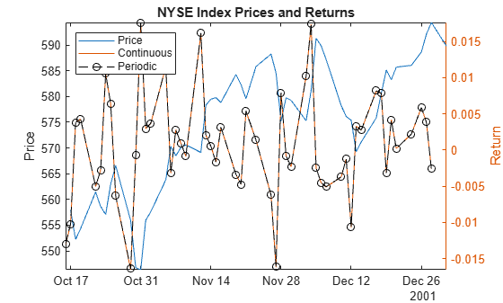
figure
plot(dates(idx + 1),TT.NASDAQ(idx + 1))
title("NASDAQ Index Prices and Returns")
ylabel("Price")
yyaxis right
h = plot(dates(idx),[TTRetC.NASDAQ(idx) TTRetP.NASDAQ(idx)]);
h(2).Marker = 'o';
h(2).Color = 'k';
ylabel("Return")
legend(["Price" "Continuous" "Periodic"],Location="northwest")
axis tight

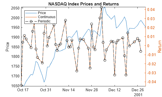
In this case, the simple periodic and continuously compounded returns of each price series are similar.

Specify Observation Times and Units

Create two stock price series from continuously compounded returns that have the following characteristics:

• Series 1 grows at a 10 percent rate at each observation time.

• Series 2 changes at a random uniform rate in the interval [-0.1, 0.1] at each observation time.

• Each series starts at price 100 and is 10 observations in length.

rng(1); % For reproducibility
numObs = 10;
p1 = 100;
r1 = 0.10;
r2 = [0; unifrnd(-0.10,0.10,numObs - 1,1)];

s1 = 100*exp(r1*(0:(numObs - 1))');
cr2 = cumsum(r2);
s2 = 100*exp(cr2);
S = [s1 s2];

Convert each price series to a return series, and return the observation intervals.

[R,intervals] = price2ret(S);

Prepend the return series so that the input and output elements are of the same length and correspond.

[[NaN; intervals] S [[NaN NaN]; R] r2]

ans = 10×6

       NaN  100.0000  100.0000       NaN       NaN         0
    1.0000  110.5171   98.3541    0.1000   -0.0166   -0.0166
    1.0000  122.1403  102.7850    0.1000    0.0441    0.0441
    1.0000  134.9859   93.0058    0.1000   -0.1000   -0.1000
    1.0000  149.1825   89.4007    0.1000   -0.0395   -0.0395
    1.0000  164.8721   83.3026    0.1000   -0.0706   -0.0706
    1.0000  182.2119   76.7803    0.1000   -0.0815   -0.0815
    1.0000  201.3753   72.1105    0.1000   -0.0627   -0.0627
    1.0000  222.5541   69.9172    0.1000   -0.0309   -0.0309
    1.0000  245.9603   68.4885    0.1000   -0.0206   -0.0206

price2ret returns rates matching the rates from the simulated series. price2ret assumes prices are recorded in a regular time base. Therefore, all durations between prices are 1.

Convert the prices to returns again, but associate the prices with years starting from August 1, 2010.

tau1 = datetime(2010,08,01);
dates = tau1 + years((0:(numObs-1))');
[Ry,intervalsy] = price2ret(S,Ticks=dates);
[[NaN; intervalsy] S [[NaN NaN]; Ry] r2]

ans = 10×6

       NaN  100.0000  100.0000       NaN       NaN         0
  365.2425  110.5171   98.3541    0.0003   -0.0000   -0.0166
  365.2425  122.1403  102.7850    0.0003    0.0001    0.0441
  365.2425  134.9859   93.0058    0.0003   -0.0003   -0.1000
  365.2425  149.1825   89.4007    0.0003   -0.0001   -0.0395
  365.2425  164.8721   83.3026    0.0003   -0.0002   -0.0706
  365.2425  182.2119   76.7803    0.0003   -0.0002   -0.0815
  365.2425  201.3753   72.1105    0.0003   -0.0002   -0.0627
  365.2425  222.5541   69.9172    0.0003   -0.0001   -0.0309
  365.2425  245.9603   68.4885    0.0003   -0.0001   -0.0206

price2ret assumes time units are days. Therefore, all durations are approximately 365 and the returns are normalized for that time unit.

Compute returns again, but specify that the observation times are years.

[Ryy,intervalsyy] = price2ret(S,Ticks=dates,Units="years");
[[NaN; intervalsyy] S [[NaN NaN]; Ryy] r2]

ans = 10×6

       NaN  100.0000  100.0000       NaN       NaN         0
    1.0000  110.5171   98.3541    0.1000   -0.0166   -0.0166
    1.0000  122.1403  102.7850    0.1000    0.0441    0.0441
    1.0000  134.9859   93.0058    0.1000   -0.1000   -0.1000
    1.0000  149.1825   89.4007    0.1000   -0.0395   -0.0395
    1.0000  164.8721   83.3026    0.1000   -0.0706   -0.0706
    1.0000  182.2119   76.7803    0.1000   -0.0815   -0.0815
    1.0000  201.3753   72.1105    0.1000   -0.0627   -0.0627
    1.0000  222.5541   69.9172    0.1000   -0.0309   -0.0309
    1.0000  245.9603   68.4885    0.1000   -0.0206   -0.0206

price2ret normalizes the returns relative to years, and now the returned rates match the simulated rates.

Input Arguments

Prices — Time series of prices

numeric matrix

Time series of prices, specified as a numObs-by-numVars numeric matrix. Each row of Prices corresponds to an observation time specified by the optional Ticks name-value argument. Each column of Prices corresponds to an individual price series.

Data Types: double

PriceTbl — Time series of prices

table | timetable

Time series of prices, specified as a table or timetable with numObs rows. Each row of Tbl is an observation time. For a table, the optional Ticks name-value argument specifies observation times. For a timetable, PriceTbl.Time specifies observation times and it must be a datetime vector.

Specify numVars variables, from which to compute returns, by using the DataVariables argument. The selected variables must be numeric.

Name-Value Arguments

Specify optional pairs of arguments as Name1=Value1,...,NameN=ValueN, where Name is the argument name and Value is the corresponding value. Name-value arguments must appear after other arguments, but the order of the pairs does not matter.

Before R2021a, use commas to separate each name and value, and enclose Name in quotes.

Example: price2ret(Tbl,Method="periodic",DataVariables=1:5) computes the simple periodic returns of the first five variables in the input table Tbl.

Ticks — Observation times τ

numeric vector | datetime vector

Observation times τ, specified as a length numObs numeric or datetime vector of increasing values.

When the input price series are in a matrix or table, the default is 1:numObs.

When the input price series are in a timetable, price2ret uses the row times in PriceTbl.Time and ignores Ticks. PriceTbl.Time must be a datetime vector.

Example: Ticks=datetime(1950:2020,12,31) specifies the end of each year from 1950 through 2020.

Example: Ticks=datetime(1950,03,31):calquarters(1):datetime(2020,12,31) specifies the end of each quarter during the years 1950 through 2020.

Data Types: double | datetime

Units — Time units

"days" (default) | "milliseconds" | "seconds" | "minutes" | "hours" | "years" | character vector

Time units to use when observation times Ticks are datetimes, specified as a value in this table.

Value	Description
"milliseconds"	Milliseconds
"seconds"	Seconds
"minutes"	Minutes
"hours"	Hours
"days"	Days
"years"	Years

price2ret requires time units to convert duration intervals to numeric values for normalizing returns.

When the value of the Ticks name-value argument is a numeric vector, price2ret ignores the value of Units.

Example: Units="years"

Data Types: char | string

Method — Compounding method

"continuous" (default) | "periodic" | character vector

Compounding method, specified as a value in this table.

Value	Description
"continuous"	Compute continuously compounded returns
"periodic"	Compute simple periodic returns

Example: Method="periodic"

Data Types: char | string

DataVariables — Variables in PriceTbl

all variables (default) | string vector | cell vector of character vectors | vector of integers | logical vector

Variables in PriceTbl, from which price2ret computes returns, specified as a string vector or cell vector of character vectors containing variable names in PriceTbl.Properties.VariableNames, or an integer or logical vector representing the indices of names. The selected variables must be numeric.

Example: DataVariables=["GDP" "CPI"]

Example: DataVariables=[true true false false] or DataVariables=[1 2] selects the first and second table variables.

Data Types: double | logical | char | cell | string

Output Arguments

Returns — Return series

numeric matrix

Return series, returned as a (numObs – 1)-by-numVars numeric matrix. price2ret returns Returns when you supply the input Prices.

Returns in row i r_i are associated with price interval [p_i,p_i+1], i = 1:(numObs - 1), according to the compounding method Method:

• When Method is "continuous",

  $$r_i=\frac{\log \left(p_{i+1}/p_i\right)}{{\tau }_{i+1}-{\tau }_i}.$$

• When Method is "periodic",

  $$r_i=\frac{\left(p_{i+1}/p_i\right)-1}{{\tau }_{i+1}-{\tau }_i}.$$

When observation times τ (see Ticks) are datetimes, the magnitude of the normalizing interval τ_i+1 – τ_i depends on the specified time units (see Units).

intervals — Time intervals between observations

numeric vector

Time intervals between observations τ_i+1 – τ_i, returned as a length numObs – 1 numeric vector. price2ret returns intervals when you supply the input Prices.

When observation times (see Ticks) are datetimes, interval magnitudes depend on the specified time units (see Units).

ReturnTbl — Return series and time intervals

table | timetable

Return series and time intervals, returned as a table or timetable, the same data type as PriceTbl, with numObs – 1 rows. price2ret returns ReturnTbl when you supply the input PriceTbl.

ReturnTbl contains the outputs Returns and intervals.

ReturnTbl associates observation time τ_i+1 with the end of the interval for the returns in row i r_i.

Algorithms

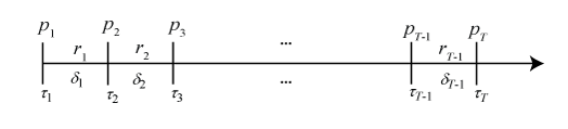
Consider the following variables:

• p is a price series (Prices).

• r is the corresponding return series (Returns).

• τ is a vector of the observation times (Ticks).

• δ is the series of lengths between observation times (intervals).

The following figure shows how the inputs and outputs are associated.

Version History

Introduced before R2006a

R2022a: price2ret supports name-value argument syntax for all optional inputs

price2ret accepts the observation times ticktimes and compounding method method as the name-value arguments Ticks and Method, respectively. However, the function will continue to accept the previous syntax.

The syntax before R2022a is

price2ret(Prices,ticktimes,method)

The recommended syntax for R2022a and later releases is

price2ret(Prices,Ticks=ticktimes,Method=method)

As with any set of name-value arguments, you can specify them in any order.