ret2price
Convert returns to prices
Syntax
Description
PriceTbl = ret2price(ReturnTbl)DataVariables
name-value argument. (since R2022a)
[___] = ret2price(___,
specifies options using one or more name-value arguments in
addition to any of the input argument combinations in previous syntaxes.
Name=Value)ret2price returns the output argument combination for the
corresponding input arguments. For example,
ret2price(Tbl,Method="periodic",DataVariables=1:5) computes prices from
the simple periodic returns in the first five variables in the input table
Tbl. (since R2022a)
Examples
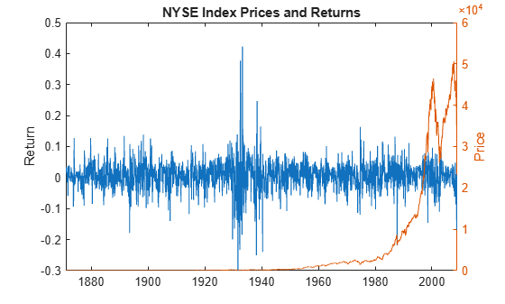
Load the Schwert Stock data set Data_SchwertStock.mat, which contains monthly returns of the NYSE index from 1871 through 2008 DataTableMth.Return, among other variables (enter Description for more details).
load Data_SchwertStock
returns = DataTableMth.Return;
numObs = numel(returns)
numObs = 1656
dates = datetime(datesMth,ConvertFrom="datenum");Set missing (NaN) returns to 0.
returns(isnan(returns)) = 0;
Convert the monthly NYSE returns to prices.
prices = ret2price(returns);
prices is a 1657-by-1 vector of monthly NYSE prices from the continuously compounded returns. ret2price sets the starting price to 1 by default; specify the StartPrice name-value argument to set an appropriate starting price.
r10 = returns(9)
r10 =
0.0114
p9_10 = [prices(9) prices(10)]
p9_10 = 1×2

    1.1274    1.1403
returns(10) = 0.0114 is the monthly return of the prices in the interval [1.1274, 1.1403].
plot(dates,DataTableMth.Return)
ylabel("Return")
yyaxis right
plot([dates(1) - month(1); dates],prices)
ylabel("Price")
title("NYSE Index Prices and Returns")
Since R2022a
Compute price series from return series, which are variables in a table. This example also shows how to convert prices in a timetable.
Load and Preprocess Data
Load the Schwert Stock data set Data_SchwertStock.mat, which contains monthly returns of several series in the table DataTableMth. Replace all missing values (NaN) with 0.
load Data_SchwertStock
DTM = fillmissing(DataTableMth,"constant",0);
Convert Returns in Table to Prices
Convert all return series in the table to prices.
PriceTbl = ret2price(DTM);
tail(PriceTbl)
    Tick    Interval    Return    DivYld    CapGain    CapGainA
    ____    ________    ______    ______    _______    ________

    1649       1        46004      16.9     5.3445      5.4712
    1650       1        42215      16.9     5.3445      5.4712
    1651       1        41801      16.9     5.3445      5.4712
    1652       1        42313      16.9     5.3445      5.4712
    1653       1        38592      16.9     5.3445      5.4712
    1654       1        32615      16.9     5.3445      5.4712
    1655       1        30263      16.9     5.3445      5.4712
    1656       1        30501      16.9     5.3445      5.4712
Because DTM is a table, PriceTbl is a table. PriceTbl contains the price series computed from the continuously compounded returns (variable names match the input variable names), observation times Tick, and time intervals Interval.
You can choose a subset of variables to convert to prices by using the DataVariables name-value argument.
Convert Returns in Timetable to Prices
Convert the table DTM to a timetable.
dates = datetime(datesMth,ConvertFrom="datenum");
TT = table2timetable(DTM,RowTimes=dates);
TT.Dates = [];
When the input series is a timetable, ret2price requires a starting time, which is specified by the StartTime name-value argument.
Convert only the NYSE and capital gain returns to prices, and specify the following options:
The starting time is exactly one month before the first observed return.
The starting prices of the NYSE and capital gains returns are 100 and 10, respectively.
The returns are periodic.
startTime = TT.Time(1) - month(1);
varnames = ["Return" "CapGain"];
startPrice = [100 10];
PriceTT = ret2price(TT,DataVariables=varnames,Method="periodic", ...
    StartTime=startTime,StartPrice=startPrice);
head(PriceTT)
       Time        Interval    Return    CapGain
    ___________    ________    ______    _______

    31-Dec-1870      NaN          100        10
    01-Jan-1871        1       101.24    10.023
    01-Feb-1871       31       164.61    14.374
    01-Mar-1871       28       301.26    24.381
    01-Apr-1871       31       619.29     46.79
    01-May-1871       30       1148.5    79.862
    01-Jun-1871       31       599.29    60.866
    01-Jul-1871       30       443.99    27.923
Because TT is a timetable, PriceTT is a timetable. PriceTT contains only those requested price series. Because the input data is time aware, the time-related variables in PriceTT contain more information about the observation times than returned when the input data is a matrix or table. For example, rather than tick times, the output timetable contains observation dates for the prices and the interval is in days.
Since R2022a
Create two stock price series from continuously compounded returns that have the following characteristics:
Series 1 grows at a 10 percent rate at each observation time.
Series 2 changes at a random uniform rate in the interval [-0.1, 0.1] at each observation time.
Each series starts at price 100 and is 10 observations in length.
rng(1); % For reproducibility
numObs = 10;
p1 = 100;
r1 = 0.10;
r2 = [0; unifrnd(-0.10,0.10,numObs - 1,1)];

s1 = 100*exp(r1*(0:(numObs - 1))');
cr2 = cumsum(r2);
s2 = 100*exp(cr2);
S = [s1 s2];
Convert each price series to a return series, and return the observation intervals.
[R,intervals] = price2ret(S);
Prepend the return series so that the input and output elements are of the same length and correspond.
[[NaN; intervals] S [[NaN NaN]; R] r2]
ans = 10×6

       NaN  100.0000  100.0000       NaN       NaN         0
    1.0000  110.5171   98.3541    0.1000   -0.0166   -0.0166
    1.0000  122.1403  102.7850    0.1000    0.0441    0.0441
    1.0000  134.9859   93.0058    0.1000   -0.1000   -0.1000
    1.0000  149.1825   89.4007    0.1000   -0.0395   -0.0395
    1.0000  164.8721   83.3026    0.1000   -0.0706   -0.0706
    1.0000  182.2119   76.7803    0.1000   -0.0815   -0.0815
    1.0000  201.3753   72.1105    0.1000   -0.0627   -0.0627
    1.0000  222.5541   69.9172    0.1000   -0.0309   -0.0309
    1.0000  245.9603   68.4885    0.1000   -0.0206   -0.0206
price2ret returns rates matching the rates from the simulated series. price2ret assumes prices are recorded in a regular time base, therefore all durations between prices are 1.
Convert the prices to returns again, but associate the prices with years starting from August 1, 2010.
tau1 = datetime(2010,08,01);
dates = tau1 + years((0:(numObs-1))');
[Ry,intervalsy] = price2ret(S,Ticks=dates);
[[NaN; intervalsy] S [[NaN NaN]; Ry] r2]
ans = 10×6

       NaN  100.0000  100.0000       NaN       NaN         0
  365.2425  110.5171   98.3541    0.0003   -0.0000   -0.0166
  365.2425  122.1403  102.7850    0.0003    0.0001    0.0441
  365.2425  134.9859   93.0058    0.0003   -0.0003   -0.1000
  365.2425  149.1825   89.4007    0.0003   -0.0001   -0.0395
  365.2425  164.8721   83.3026    0.0003   -0.0002   -0.0706
  365.2425  182.2119   76.7803    0.0003   -0.0002   -0.0815
  365.2425  201.3753   72.1105    0.0003   -0.0002   -0.0627
  365.2425  222.5541   69.9172    0.0003   -0.0001   -0.0309
  365.2425  245.9603   68.4885    0.0003   -0.0001   -0.0206
price2ret assumes time units are days. Therefore, all durations are approximately 365 and the returns are normalized for that time unit.
Compute returns again, but specify that the observation times are years.
[Ryy,intervalsyy] = price2ret(S,Ticks=dates,Units="years");
[[NaN; intervalsyy] S [[NaN NaN]; Ryy] r2]
ans = 10×6
NaN 100.0000 100.0000 NaN NaN 0
1.0000 110.5171 98.3541 0.1000 -0.0166 -0.0166
1.0000 122.1403 102.7850 0.1000 0.0441 0.0441
1.0000 134.9859 93.0058 0.1000 -0.1000 -0.1000
1.0000 149.1825 89.4007 0.1000 -0.0395 -0.0395
1.0000 164.8721 83.3026 0.1000 -0.0706 -0.0706
1.0000 182.2119 76.7803 0.1000 -0.0815 -0.0815
1.0000 201.3753 72.1105 0.1000 -0.0627 -0.0627
1.0000 222.5541 69.9172 0.1000 -0.0309 -0.0309
1.0000 245.9603 68.4885 0.1000 -0.0206 -0.0206
price2ret normalizes the returns relative to years, and now the returned rates match the simulated rates.
Complete the roundtrip by converting all returns series back to prices. Specify the returned observation intervals and the starting prices p1.
[P,ticks] = ret2price(R,Intervals=intervals,StartPrice=p1);
[Py,ticksy] = ret2price(Ry,Intervals=intervalsy,StartPrice=p1);
[Pyy,ticksyy] = ret2price(Ryy,Intervals=intervalsyy,StartPrice=p1,Units="years");

[ticks ticksy ticksyy]
ans = 10×3
103 ×
0 0 0
0.0010 0.3652 0.0010
0.0020 0.7305 0.0020
0.0030 1.0957 0.0030
0.0040 1.4610 0.0040
0.0050 1.8262 0.0050
0.0060 2.1915 0.0060
0.0070 2.5567 0.0070
0.0080 2.9219 0.0080
0.0090 3.2872 0.0090
[S P Py Pyy]
ans = 10×8

  100.0000  100.0000  100.0000  100.0000  100.0000  100.0000  100.0000  100.0000
  110.5171   98.3541  110.5171   98.3541  110.5171   98.3541  110.5171   98.3541
  122.1403  102.7850  122.1403  102.7850  122.1403  102.7850  122.1403  102.7850
  134.9859   93.0058  134.9859   93.0058  134.9859   93.0058  134.9859   93.0058
  149.1825   89.4007  149.1825   89.4007  149.1825   89.4007  149.1825   89.4007
  164.8721   83.3026  164.8721   83.3026  164.8721   83.3026  164.8721   83.3026
  182.2119   76.7803  182.2119   76.7803  182.2119   76.7803  182.2119   76.7803
  201.3753   72.1105  201.3753   72.1105  201.3753   72.1105  201.3753   72.1105
  222.5541   69.9172  222.5541   69.9172  222.5541   69.9172  222.5541   69.9172
  245.9603   68.4885  245.9603   68.4885  245.9603   68.4885  245.9603   68.4885
Input Arguments
Name-Value Arguments
Output Arguments
Algorithms
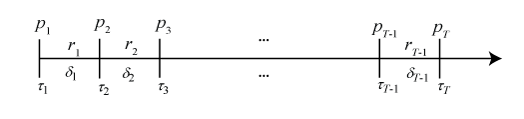
Consider the following variables:
The following figure shows how the inputs and outputs are associated.