Decompose Time Series Into Additive Trend Components
This example shows how to estimate nonseasonal and seasonal trend components using parametric models. For details on trend components of a time series, see internal link.
The sample data is a time series of monthly accidental deaths in the U.S. from 1973 to 1978 (Brockwell and Davis, 2002).
Load Data
Load the accidental deaths data set.
load Data_Accidental
y = DataTimeTable.NUMD;
T = length(y);

figure
plot(DataTimeTable.Time,y/1000)
title('Monthly Accidental Deaths')
ylabel('Number of Deaths (thousands)')
hold on
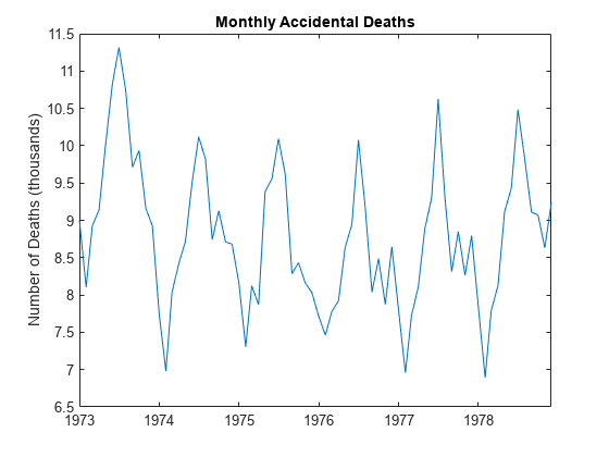
The data shows a potential quadratic trend and a strong seasonal component with periodicity 12.
Fit Quadratic Trend
Fit the polynomial
to the observed series.
t = (1:T)';
X = [ones(T,1) t t.^2];

b = X\y;
tH = X*b;

h2 = plot(DataTimeTable.Time,tH/1000,'r','LineWidth',2);
legend(h2,'Quadratic Trend Estimate')
hold off
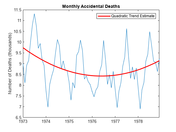
Detrend Original Series
Subtract the fitted quadratic line from the original data.
xt = y - tH;
Estimate Seasonal Indicator Variables
Create indicator (dummy) variables for each month. The first indicator is equal to one for January observations, and zero otherwise. The second indicator is equal to one for February observations, and zero otherwise. A total of 12 indicator variables are created for the 12 months. Regress the detrended series against the seasonal indicators.
mo = repmat((1:12)',6,1);
sX = dummyvar(mo);

bS = sX\xt;
st = sX*bS;

figure
plot(DataTimeTable.Time,st/1000)
ylabel 'Number of Deaths (thousands)';
title('Parametric Estimate of Seasonal Component (Indicators)')
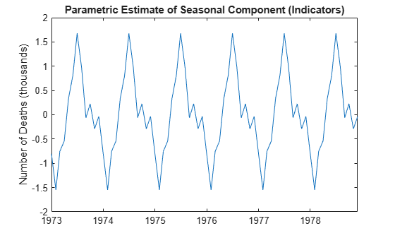
In this regression, all 12 seasonal indicators are included in the design matrix. To prevent collinearity, an intercept term is not included (alternatively, you can include 11 indicators and an intercept term).
Deseasonalize Original Series
Subtract the estimated seasonal component from the original series.
dt = y - st;

figure
plot(DataTimeTable.Time,dt/1000)
title('Monthly Accidental Deaths (Deseasonalized)')
ylabel('Number of Deaths (thousands)')
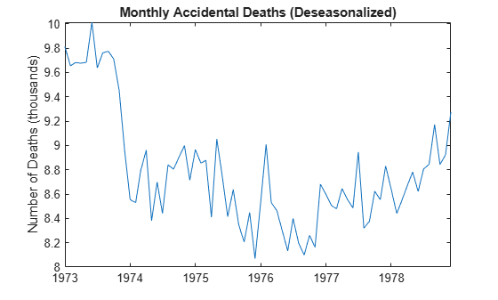
The quadratic trend is much clearer with the seasonal component removed.
Estimate Irregular Component
Subtract the trend and seasonal estimates from the original series. The remainder is an estimate of the irregular component.
bt = y - tH - st;

figure
plot(DataTimeTable.Time,bt/1000)
title('Irregular Component')
ylabel('Number of Deaths (thousands)')
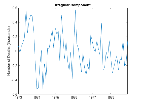
You can optionally model the irregular component using a stochastic process model.
What is Time Series Decomposition
Time series decomposition involves separating a time series into several distinct components. In most cases, time series are decomposed into three components:
— Deterministic, nonseasonal secular trend component. Usually, this component is a linear trend, but higher-degree polynomials are possible.
— Deterministic seasonal component with known periodicity. This component captures level shifts that repeat systematically within the same period (e.g., month or quarter) between successive years. Often, is considered a nuisance component; you can eliminate it by applying a seasonal adjustment.
— Stochastic irregular component. This component is not necessarily a white noise process; it can exhibit autocorrelation and cycles of unpredictable duration. As a result, this component might contain information about the business cycle.
The following functional forms are most often used to represent a time series as a function of its trend, seasonal, and irregular components:
Additive Decomposition — . This form is the classical decomposition, appropriate when the series has no exponential growth and the amplitude of the seasonal component is constant over time. For identifiability from the trend component, the seasonal and irregular components are assumed to fluctuate around zero.
Multiplicative Decomposition — . This decomposition is appropriate when the series exhibits exponential growth and the amplitude of the seasonal component grows with the level of the series. For identifiability from the trend component, the seasonal and irregular components are assumed to fluctuate around one.
Log-additive decomposition — . This decomposition is an alternative to the multiplicative decomposition. If has a multiplicative decomposition, the logged series has an additive decomposition. This decomposition is well suited when is positive and has many values that are close to 0. For identifiability from the trend component, the seasonal and irregular components are assumed to fluctuate around zero.
You can estimate the trend and seasonal components by using filters (moving averages) or parametric regression models. Given estimates and , the irregular component is estimated as using the additive decomposition, and using the multiplicative decomposition.
The series (or using the multiplicative decomposition) is a detrended series. Similarly, the series (or using the multiplicative decomposition) is called a deseasonalized series.
See Also
dummyvar | hpfilter | bkfilter | cffilter | hfilter
Topics
- Data Transformations
- Use Hodrick-Prescott Filter to Reproduce Original Result
- Choose Time Series Filter for Business Cycle Analysis
- Estimate Moving Average Trend Using Moving Average Filter
- Seasonal Adjustment Using a Stable Seasonal Filter
- Seasonal Adjustment Using S(n,m) Seasonal Filters
- Seasonal Adjustment