Detect Serial Correlation Using Econometric Modeler App
These examples show how to assess serial correlation by using the
Econometric Modeler app. Methods include plotting the autocorrelation function (ACF) and
partial autocorrelation function (PACF), and testing for significant lag coefficients
using the Ljung-Box Q-test. The data set Data_Overshort.mat contains
57 consecutive days of overshorts from a gasoline tank in Colorado.
Plot ACF and PACF
This example shows how to plot the ACF and PACF of a time series.
Download the Data_Overshort.mat MAT-file into your current folder, and then
load it into the workspace.
fldr = pwd;
openExample("Data_Overshort.mat",workDir=fldr);
load(fullfile(fldr,"Data_Overshort.mat"))
To change the folder to which to download the data set, set fldr to its absolute path.
At the command line, open the Econometric Modeler app.
econometricModeler
Alternatively, open the app from the apps gallery (see Econometric Modeler).
Import DataTable into the app:
On the Modeler tab, in the Import section, click the Import button
 .
.In the Import Data dialog box, select the check box for the
DataTablevariable.Click Import.
The variable OSHORT appears in the
Time Series pane, and its time series plot appears
in the Plot(OSHORT) figure window.
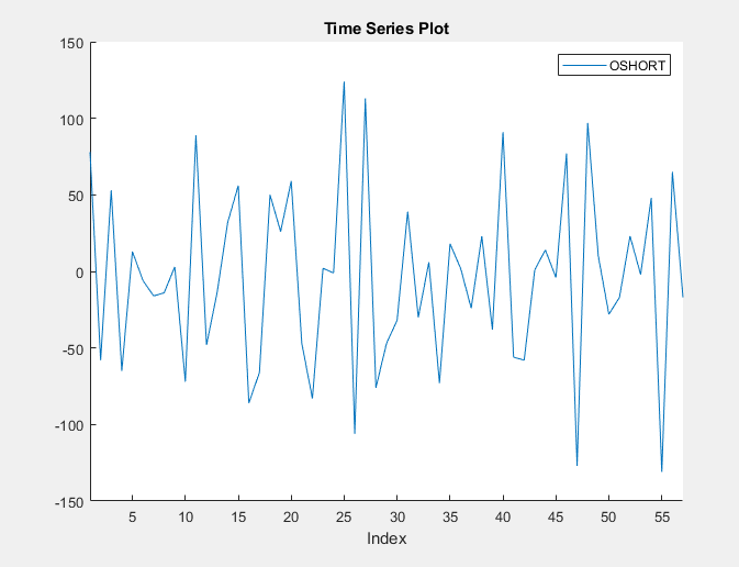
The series appears to be stationary.
Close the Plot(OSHORT) figure window.
Plot the ACF of OSHORT by clicking the
Plots tab. The ACF appears in the
ACF(OSHORT) figure window then clicking
ACF.
Plot the PACF of OSHORT by clicking the
Plots tab then clicking PACF.
The PACF appears in the PACF(OSHORT) figure
window.
Position the correlograms so that you can view them at the same time by dragging the PACF(OSHORT) figure window to the bottom of the right pane.
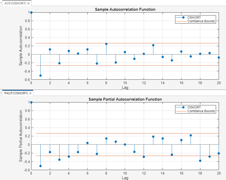
The sample ACF and PACF exhibit significant autocorrelation (that is, both contain lags that are more than two standard deviations away from 0). The sample ACF shows that the autocorrelation at lag 1 is significant. The sample PACF shows that the autocorrelations at lags 1, 3, and 4 are significant.
The distinct cutoff of the ACF and the more gradual decay of the PACF suggest an MA(1) model might be appropriate for this data.
Conduct Ljung-Box Q-Test for Significant Autocorrelation
This example shows how to conduct the Ljung-Box Q-test for significant autocorrelation lags.
Download the Data_Overshort.mat MAT-file into your current folder, and then
load it into the workspace.
fldr = pwd;
openExample("Data_Overshort.mat",workDir=fldr);
load(fullfile(fldr,"Data_Overshort.mat"))
To change the folder to which to download the data set, set fldr to its absolute path.
At the command line, open the Econometric Modeler app.
econometricModeler
Alternatively, open the app from the apps gallery (see Econometric Modeler).
Import DataTimeTable into the app:
On the Modeler tab, in the Import section, click the Import button
.In the Import Data dialog box, select the check box for the
DataTimeTablevariable.Click Import.
The variable OSHORT appears in the
Time Series pane, and its time series plot appears
in the Plot(OSHORT) figure window.
The series appears to be stationary, and it fluctuates around a constant mean. Therefore, you do not need to transform the data before conducting the test.
Conduct three Ljung-Box Q-Tests for testing the null hypothesis that the first 10, 5, and 1 autocorrelations are jointly zero:
On the Modeler tab, in the Tests section, click Add Test > Ljung-Box Q-Test.
On the LBQ tab, in the Settings section:
Set Number of Lags to
10.Set DOF to
10.To achieve a false positive rate below 0.05, use the Bonferroni correction to set Significance Level to 0.05/3 =
0.0167.
In the Tests section, click Run Test.
Repeat steps 2 and 3 twice, with these changes:
Set Number of Lags to
5and the DOF to5.Set Number of Lags to
1and the DOF to1.
The test results appear in the Results table of the LBQ(OSHORT) document.
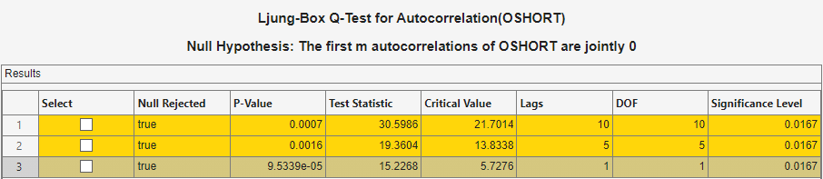
The results show that not every autocorrelation up to lag 5 (or 10) is zero, indicating volatility clustering in the residual series.
See Also
Apps
Functions
Topics
- Detect Autocorrelation
- Analyze Time Series Data Using Econometric Modeler
- Prepare Time Series Data for Econometric Modeler App
- Plot Time Series Data Using Econometric Modeler App
- Detect ARCH Effects Using Econometric Modeler App
- Programmatically Select ARIMA Model for Time Series Using Box-Jenkins Methodology
- Autocorrelation and Partial Autocorrelation
- Implement Box-Jenkins Model Selection and Estimation Using Econometric Modeler App
- Creating ARIMA Models Using Econometric Modeler App