Filter Visualizer
Libraries:
DSP System Toolbox /
Sinks
Description
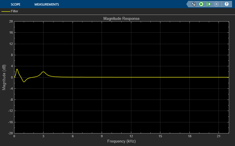
The Filter Visualizer block displays the magnitude response and phase response of time-varying digital filters or time-varying filter coefficients. You can visualize the frequency response of up to 20 filters at a time using this visualizer.
You can use the visualizer to configure the plot settings, find the peak values, enable
cursor measurements, and even copy the scope display to the clipboard For more information,
see Configure Filter Visualizer. To access the filter
visualizer programmatically, use the dsp.DynamicFilterVisualizer object.
Examples
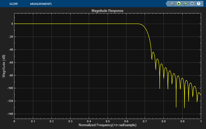
Vary the order and the cutoff frequency of the lowpass FIR filter during simulation. Design the filter every time the frequency specifications update. Visualize the magnitude response of this varying filter.
Pass a noisy sinusoidal signal through the lowpass FIR filter. Visualize the frequency spectra of the input and the output signals.
Open and Inspect Model
Open the tunable_lowpass_filter model.
The input signal in the model is a sum of two sine waves with the frequencies of 1 kHz and 15 kHz. The Random Source block adds zero-mean white Gaussian noise with a variance of 0.05 to the sum of sine waves.
The Lowpass FIR Filter Design block designs the filter and the Discrete FIR Filter block implements the filter. The filter order and the filter cutoff frequency specifications are input through the input ports of the Lowpass FIR Filter Design block.
Run Model
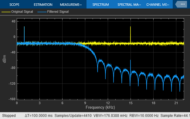
Visualize the spectra of the original signal and the filtered signal in the Spectrum Analyzer. The second tone at 15 kHz is attenuated since it falls in the stopband region of the filter.

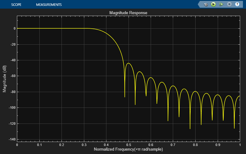
Tune the Filter Order and Filter Cutoff Frequency
Change the filter order to 90 and the filter cutoff frequency to 0.7 during simulation. To change the parameter values more gradually during simulation, select the Smooth tuned filter parameters check box and specify a smoothing factor in the Lowpass FIR Filter Design block dialog box. The smoothing factor determines the speed at which the parameter values change until they match the desired new value. If you specify a smoothing factor of 0, the block does not smooth the parameter and immediately sets the parameter to the new value. As the smoothing factor approaches 1, the number of smoothing operations, and consequently, the number of filter redesigns increase. This example uses a smoothing factor of 0.6.
When you change the filter order and the filter cutoff frequency, you can see the magnitude response of the filter change in the Filter Visualizer output. The second tone at 15 kHz is now unaffected as it falls in the passband region of the filter.

Filter a noisy sinusoidal signal using the Fourth-Order Section Filter block. Obtain the numerator and denominator coefficients of the FOS filter using the Bandpass IIR Filter Design block.
Tune the frequency specifications of the FOS filter during simulation.
Open and Run Model
Open the fourthordersectionfilter.slx model.
The input signal in the model is a sum of two sine waves with frequencies of 100 Hz and 350 Hz. The sample rate is 1000 Hz and the number of samples in each frame is 1024. The Random Source block adds zero-mean white Gaussian noise with a variance of 1e-4 to the sum of the sine waves.
The Bandpass IIR Filter Design block designs a sixth-order bandpass IIR filter with the first and second 3-dB cutoff frequencies of 0.25  rad/sample and 0.75 rad/sample, respectively. The block generates coefficients as a cascade of fourth-order sections. Visualize the frequency response of the filter using the Filter Visualizer.
Run the model.
The Fourth-Order Section Filter block filters the noisy sinusoidal signal. Visualize the original sinusoidal signal and the filtered signal using the spectrum analyzer.


Tune Frequency Specification of FOS Filter
During simulation, you can tune the frequency specifications of the FOS filter by tuning the frequency parameters in the Bandpass IIR Filter Design block. The frequency response of the FOS filter updates accordingly.
Change the first 3-dB cutoff frequency to 0.65 rad/sample in the Bandpass IIR Filter Design block. The first tone of the sinusoidal signal is attenuated as it no longer falls in the passband region of the filter.


Filter a noisy sinusoidal signal using the Second-Order Section Filter block. Obtain the numerator and denominator coefficients of the SOS filter using the Bandstop IIR Filter Design block.
Tune the frequency specifications of the SOS filter during simulation.
Open and Run Model
Open the secondordersection_bandstopfilter model.
The input signal in the model is a sum of two sine waves with the frequencies of 200 Hz and 400 Hz. The sample rate is 1000 Hz and the number of samples in each frame is 1024. The Random Source block adds zero-mean white Gaussian noise with a variance of 1e-4 to the sum of the sine waves.
The Bandstop IIR Filter Design block designs a sixth-order bandstop IIR filter with the first and second 3-dB cutoff frequencies of 0.2  rad/sample and 0.75 rad/sample, respectively. The block generates coefficients as a cascade of second-order sections. Visualize the frequency response of the filter using Filter Visualizer.
Run the model.
The Second-Order Section Filter block filters the noisy sinusoidal signal. Visualize the original sinusoidal signal and the filtered signal using the Spectrum Analyzer. The first tone is attenuated as it falls in the stopband region of the filter while the second tone remains unaffected as it falls in the passband region of the filter.


Tune Frequency Specification of SOS Filter
During simulation, you can tune the frequency specifications of the SOS filter by tuning the frequency parameters in the Bandstop IIR Filter Design block. The frequency response of the SOS filter updates accordingly.
Change the first 3-dB cutoff frequency to 0.5 rad/sample in the Bandstop IIR Filter Design block. The first tone of the sinusoidal signal now falls in the passband region and is therefore unattenuated.


Extended Examples
Parametric Audio Equalizer
Model an algorithm specification for a three band parametric equalizer

System Identification Using RLS Adaptive Filtering
Use a recursive least-squares (RLS) filter to identify an unknown system modeled with a lowpass FIR filter. Use the dynamic filter visualizer to compare the frequency response of the unknown and estimated systems. This example allows you to dynamically tune key simulation parameters using a user interface (UI). The example also shows you how to use MATLAB Coder™ to generate code for the algorithm and accelerate the speed of its execution.
Ports
Input
Parameters
Scope Tab
Configuration
Specify the number of filters to display as a positive integer in the range [1 20]. The value of this parameter determines the number of input ports on the block.
Programmatic Use
Block Parameter:
NumFilters |
| Type: character vector or string scalar |
| Values: scalar in the range [1 20] |
Specify the filter response type as one of these options:
FIR— The block displays one input port per filter. You input the numerator coefficients of the filter(s) through the port(s).IIR— The block displays two input ports per filter. You input the numerator and the denominator coefficients of the filter(s) through the ports.
Programmatic Use
Block Parameter:
FilterType |
| Type: character vector or string scalar |
Values:
'FIR', 'IIR' |
Select this option to display the legend on the plot. The legend contains the
filter names in the format
Filter:. If you are visualizing
only one filter, the legend displays NumberFilter. If you are visualizing
the magnitude and phase responses of multiple filters, the visualizer displays a
separate legend for each response in the format
mag(Filter: and
Number)phase(Filter:, respectively.
If you are visualizing the responses of only one filter, the legend displays
Number)mag(Filter) and phase(Filter).
You can control which filters are visible in the scope using the legend. Click a
filter name in the legend to hide the frequency response of that filter in the scope.
To display the filter response, click the filter name again. To display only one
filter response, right-click the name of that filter, which hides all other filter
responses. To show all filter responses, press Esc. This setting is
equivalent to changing the Visible parameter in the
Scope tab > Settings (![]() ) > Color and Styling.
) > Color and Styling.
Programmatic Use
Block Parameter:
ShowLegend |
Type:boolean |
Tunable: Yes
Click the button to plot the magnitude and phase response of the filter on two separate axes. Click the button again to plot only the magnitude response.
Tunable: Yes
Programmatic Use
Block Parameter:
PlotAsMagnitudePhase |
Type:boolean |
Configuration> Filter Visualizer Settings ( )
)
Specify the number of frequency points over which to compute the spectral estimate as a positive integer.
Tunable: Yes
Programmatic Use
Block Parameter:
NumFrequencyPoints |
| Type: character vector or string scalar |
| Values: scalar |
Select this parameter to display the frequency response of the filter in normalized frequency units.
When you select this parameter, the frequency range is [0,1] and the frequency
axis (x-axis) units switch to Normalized Frequency (×π
rad/sample).
When you clear this parameter, the frequency range is [0 Fs/2] and the frequency axis (x-axis) units are in Hz.
Tunable: Yes
Programmatic Use
Block Parameter:
NormalizedFrequency |
Type:boolean |
Enter the sample rate as a positive scalar in Hz.
Tunable: Yes
Dependencies
To enable this parameter, clear the Normalized Frequency parameter.
Programmatic Use
Block Parameter:
SampleRate |
| Type: character vector or string scalar |
| Values: scalar |
Specify the frequency range as a two-element numeric vector that is monotonically increasing and of the form [fmin, fmax].
When you select the Normalized Frequency parameter, fmax is in normalized frequency units and must be a positive scalar that is less than or equal to 1. When you clear the Normalized Frequency parameter, fmax is in Hz and must be less than or equal to Fs/2, where Fs is the value you specify in the Sample Rate (Hz) parameter.
Tunable: Yes
Programmatic Use
Block Parameter:
FrequencyRange |
| Type: character vector or string |
| Value: two-element numeric vector |
Specify the magnitude units in the display as one of these:
MagnitudeMagnitude (dB)Magnitude squared
Tunable: Yes
Programmatic Use
Block Parameter:
MagnitudeDisplay |
| Type: character vector or string scalar |
Values:
'Magnitude (dB)', 'Magnitude',
'Magnitude squared' |
Since R2024b
Specify the precision of numeric values in the scope display as a positive integer in the range [1, 15].
Tunable: Yes
Specify the display title as a character vector or a string.
Tunable: Yes
Programmatic Use
Block Parameter:
Title |
| Type: character vector or string |
Specify the scale of the frequency axis as 'Linear' or
'Log'.
Tunable: Yes
Programmatic Use
Block Parameter:
XScale |
| Type: character vector or string |
Values:
'Linear', 'Log' |
Specify the y-axis limits of the magnitude display in the
Filter Visualizer as a two-element numeric vector of the form [ymin
ymax]. The units of the y-axis limits depend on the
Display Unit parameter.
Tunable: Yes
Programmatic Use
Block Parameter:
YLimits |
| Type: character vector or string |
| Value: two-element numeric vector |
Select this check box to show the grid in the Filter Visualizer display.
Tunable: Yes
Programmatic Use
Block Parameter:
ShowGrid |
Type:
logical |
Specify the type of plot to use in the filter visualizer window as one of these:
Line— The filter visualizer connects each point on the magnitude and phase response plot with a line.Stairs— The filter visualizer displays the filter response (magnitude, phase, or both) as a stair-step graph. A stair-step graph is made up of only horizontal lines and vertical lines. Each horizontal line represents the filter response over a frequency value and is connected to two vertical lines. Each vertical line represents a change in values occurring at a frequency.Stem— The filter visualizer displays the frequency response as circles with vertical lines extending down to the x-axis at each of the frequency values.
You can individually control the type of plot for each filter response curve. To control the type of plot for each curve, select the filter and set the Plot Type parameter accordingly. If you display both the magnitude and phase responses, the visualizer applies the same plot type setting to both the response curves. (since R2025a)
Tunable: Yes
Programmatic Use
Block Parameter:
PlotType |
| Type: character vector or string scalar |
Values:
'Stem', 'Line',
'Stairs' |
Specify the font size as a positive scalar in the range [1,100].
Tunable: Yes
Programmatic Use
Block Parameter:
- |
| Type: double |
Specify the color that you want to apply to the background of the scope figure.
Tunable: Yes
Specify the color that you want to apply to the background of the axes.
Tunable: Yes
Specify the color of the labels, grid, and the channel names in the legend.
Tunable: Yes
Select the filter for which you want to modify the visibility, line color, style, width, and marker properties.
Tunable: Yes
Specify whether the selected filter is visible. If you clear this check box, the frequency response line disappears in the display.
You can control this parameter directly from the legend. Click a filter name in the legend to hide the frequency response of the filter in the scope. To show the filter response, click the filter name again. To show only one filter response, right-click the filter name, which hides all other filter responses. To show all filter responses, press Esc.
Tunable: Yes
Programmatic Use
Block Parameter:
Visible |
Type:
logical |
Specify the line style for the selected filter response.
Tunable: Yes
Specify the line width for the selected filter response.
Tunable: Yes
Specify markers for the selected filter response to show at its data points. This parameter is similar to the Marker property for plots. You can choose any of the marker symbols from the drop-down list.
Tunable: Yes
Specify the line color for the selected filter response.
Tunable: Yes
Share
Click this button to copy the scope display to the clipboard. You can preserve the color in the display by selecting Preserve Colors in the Copy to Clipboard drop down.
When you copy the display to the clipboard using the Copy to Clipboard and the Print options in the Scope tab > Share section, select this parameter for the scope to preserve the colors.
To access Preserve Colors, click the drop-down arrow for Copy to Clipboard.
Tunable: Yes
Click this button to save the scope display as an image or a PDF or to print the display.
Measurements Tab
Channel
Choose the filter response for which you need to obtain measurements. The filter
names are in the format Filter:.
If you are visualizing only one filter, the legend displays NumberFilter.
If you are visualizing the magnitude and phase responses of multiple filters, the
visualizer displays a separate name for each response in the format
mag(Filter: and
Number)phase(Filter:, respectively.
If you are visualizing the responses of only one filter, the legend becomes
Number)mag(Filter) and phase(Filter).
Tunable: Yes
Dependency
To enable this parameter, pass some data through the scope.
Cursors
Click the Data Cursors button to enable data cursor measurements. Each cursor tracks a vertical line along the frequency response. The scope displays the difference between frequency(x) values and frequency response (y) values of the filter at the two cursors in the box between the cursors.
Tunable: Yes
Select this parameter to position the cursors on the signal data points.
Tunable: Yes
Select this parameter to lock the frequency difference between the two cursors.
Tunable: Yes
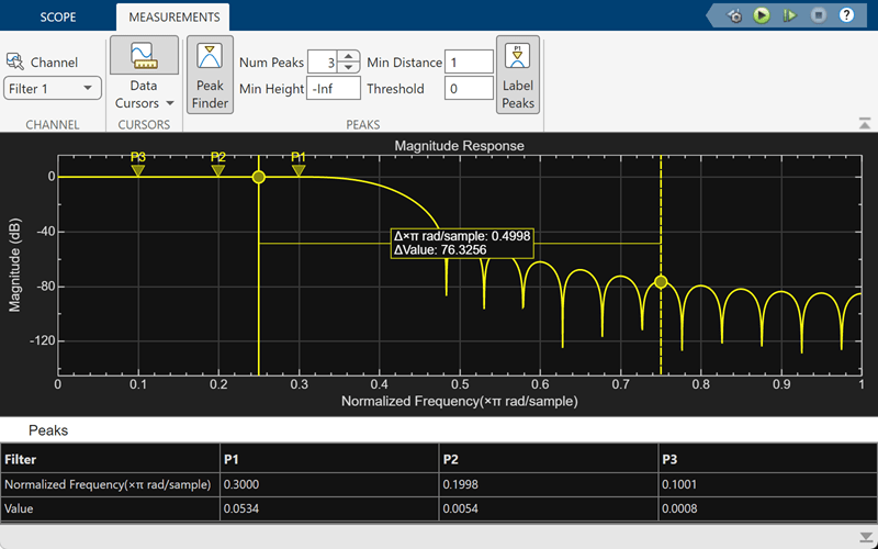
Peaks
Select Peak Finder to enable peak finder measurements. An arrow appears on the plot at each maxima and a Peaks panel appears at the bottom of the scope window.
Tunable: Yes
Specify the maximum number of peaks to show as a positive integer less than 100.
Tunable: Yes
Specify the level above which the scope detects peaks as a real scalar.
Tunable: Yes
Specify the minimum number of samples between adjacent peaks as a positive integer.
Tunable: Yes
Specify the minimum difference in the height of the peak and its neighboring samples as a nonnegative scalar.
Tunable: Yes
Select Label Peaks to label the peaks. The scope displays the labels (P1, P2, …) above the arrows in the plot.
Tunable: Yes
Property Inspector Only
Input filter names, specified as a character vector, string, or array of either.
The names appear in the legend, Filter Visualizer Settings, and
Measurements panels. If you do not specify filter names, the
block displays the filter names as Filter: 1, Filter:
2, etc.
Dependency
To see the filter names, select Legend in the Scope tab.
Programmatic Use
Block Parameter:
FilterNames |
| Type: cell array of character vectors or string array |
Auto— If you do not specify Title and y-label, maximize all plots by default.On— Maximize all plots and hide Title and y-label.Off— Do not maximize plots.
Point anywhere in the Filter Visualizer to see the maximize axes button ![]() .
.
Programmatic Use
Block Parameter:
MaximizeAxes |
| Type: character vector or string scalar |
Tunable: Yes
Auto— The filter visualizer scales the axes as needed to fit the data, both during and after simulation.Manual— The filter visualizer does not scale the axes automatically.Updates— The filter visualizer scales the axes limits once after completing the number of visual updates specified in the Number of Updates text box (100by default). Scaling occurs only once during each run.OnceAtStop— The filter visualizer scales the axes when the simulation stops.
Tunable: Yes
Programmatic Use
Block Parameter:
AxesScaling |
| Type: character vector or string scalar |
Set this property to delay auto scaling the y-axis.
Tunable: Yes
Dependency
To enable this property, set Axes Scaling to
Updates.
Programmatic Use
Block Parameter:
AxesScalingNumUpdates |
| Type: character vector or string scalar |
| Values: scalar |
Block Characteristics
Data Types |
|
Direct Feedthrough |
|
Multidimensional Signals |
|
Variable-Size Signals |
|
Zero-Crossing Detection |
|