comm.RaisedCosineTransmitFilter

Apply pulse shaping by interpolating signal using raised-cosine FIR filter

Description

The comm.RaisedCosineTransmitFilter System object™ applies pulse shaping by interpolating an input signal using a raised cosine finite impulse response (FIR) filter. The FIR filter has (FilterSpanInSymbols × OutputSamplesPerSymbol + 1) tap coefficients.

To apply pulse shaping by interpolating an input signal using a raised cosine FIR filter:

1. Create the comm.RaisedCosineTransmitFilter object and set its properties.

2. Call the object with arguments, as if it were a function.

To learn more about how System objects work, see What Are System Objects?

Creation

Syntax

txfilter = comm.RaisedCosineTransmitFilter

txfilter = comm.RaisedCosineTransmitFilter(Name,Value)

Description

txfilter = comm.RaisedCosineTransmitFilter returns a raised cosine transmit FIR filter System object, which interpolates an input signal using a raised cosine FIR filter. The filter uses an efficient polyphase FIR interpolation structure and has unit energy.

txfilter = comm.RaisedCosineTransmitFilter(Name,Value) sets properties using one or more name-value pairs. Enclose each property name in quotes. For example, comm.RaisedCosineTransmitFilter('FilterSpanInSymbols',15) configures a raised cosine transmit filter System object with the filter span set to 15 symbols.

Properties

Unless otherwise indicated, properties are nontunable, which means you cannot change their values after calling the object. Objects lock when you call them, and the release function unlocks them.

If a property is tunable, you can change its value at any time.

For more information on changing property values, see System Design in MATLAB Using System Objects.

Shape — Filter shape

'Square root' (default) | 'Normal'

Filter shape, specified as 'Square root' or 'Normal'.

Data Types: char | string

RolloffFactor — Roll-off factor

0.2 (default) | scalar in the range [0, 1]

Roll-off factor, specified as a scalar in the range [0, 1].

Data Types: double

FilterSpanInSymbols — Filter span in symbols

10 (default) | positive integer

Filter span in symbols, specified as a positive integer. The object truncates the infinite impulse response (IIR) of an ideal raised-cosine filter to an impulse response that spans the number of symbols specified by this property.

Data Types: double

OutputSamplesPerSymbol — Output samples per symbol

8 (default) | positive integer

Output samples per symbol, specified as a positive integer.

Data Types: double

Gain — Linear filter gain

1 (default) | positive scalar

Linear filter gain, specified as a positive scalar. The object designs a raised-cosine filter that has unit energy and then applies the linear filter gain to obtain final tap coefficient values.

Data Types: double

Usage

Syntax

y = txfilter(X)

Description

y = txfilter(X) applies pulse shaping by interpolating an input signal using a raised cosine FIR filter. The output consists of interpolated signal values.

Input Arguments

X — Input signal

column vector | matrix

Input signal, specified as a column vector or a K_i-by-N matrix. K_i is the number of input samples per signal channel, and N is the number of signal channels.

For a K_i-by-N matrix input, the object processes columns of the input matrix as N independent channels.

This object accepts variable-size inputs. After the object is locked, you can change the size of each input channel, but you cannot change the number of channels. For more information, see Variable-Size Signal Support with System Objects.

Data Types: double | single
Complex Number Support: Yes

Output Arguments

Y — Output signal

column vector | matrix

Output signal, returned as a column vector or a K_o-by-N matrix. K_o is equal to K_i × OutputSamplesPerSymbol. K_i is the number of input samples per signal channel, and N is the number of signal channels.

The object interpolates and filters each channel over the first dimension and then generates a K_o-by-N output matrix. The output signal is the same data type as the input signal.

Object Functions

To use an object function, specify the System object as the first input argument. For example, to release system resources of a System object named obj, use this syntax:

release(obj)

Specific to comm.RaisedCosineTransmitFilter

info	Information about filter System object
coeffs	Coefficients for filters
cost	Computational cost of implementing filter System object
freqz	Frequency response of discrete-time filter
grpdelay	Group delay response of discrete-time filter
impz	Impulse response of discrete-time filter
order	Order of discrete-time filter System object

Common to All System Objects

step	Run System object algorithm
release	Release resources and allow changes to System object property values and input characteristics
reset	Reset internal states of System object

Examples

Interpolate Signal Using Root-Raised-Cosine Filter

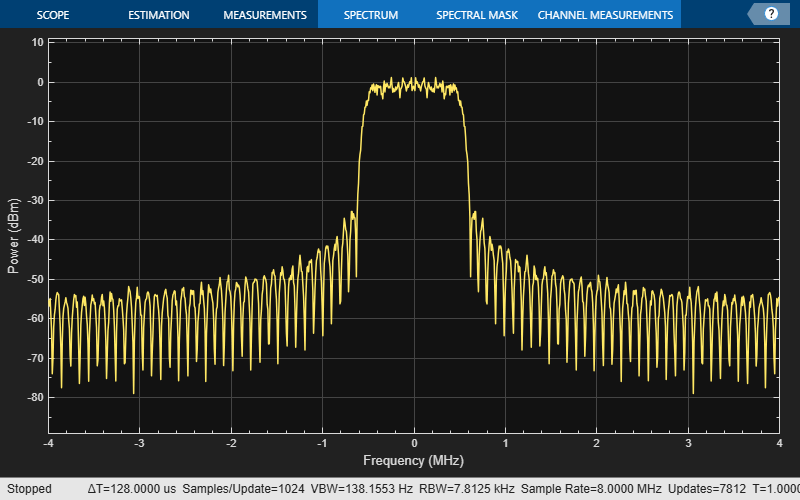
Interpolate a signal using square-root-raised-cosine (RRC) transmit filter object and display the spectrum of the filtered signal.

Create random bipolar symbols at a symbol rate of 1e6 symbols per second.

data = 2*randi([0 1],1e6,1) - 1;

Create a RRC transmit filter object. The default sets the filter to a square-root shape and the number of samples per symbol to 8.

txfilter = comm.RaisedCosineTransmitFilter

txfilter = 
  comm.RaisedCosineTransmitFilter with properties:

                     Shape: 'Square root'
             RolloffFactor: 0.2000
       FilterSpanInSymbols: 10
    OutputSamplesPerSymbol: 8
                      Gain: 1

Filter the data by using the RRC filter.

filteredData = txfilter(data);

Create a spectrum analyzer object with an 8e6 sampling rate. This sampling rate matches the sampling rate of the filtered signal.

spectrumAnalyzer = spectrumAnalyzer(SampleRate=8e6);

View the spectrum of the filtered signal by using the spectrum analyzer object.

spectrumAnalyzer(filteredData)
release(spectrumAnalyzer)

Examine Effect of Filter Span on Magnitude Response

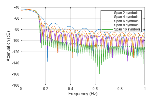
Create interpolated signals from a square-root-raised-cosine (RRC) filter with various filter spans. Examine the magnitude response of the various filter designs.

Create RRC filter objects setting various filter spans.

txfilt2 = comm.RaisedCosineTransmitFilter('FilterSpanInSymbols',2);
txfilt4 = comm.RaisedCosineTransmitFilter('FilterSpanInSymbols',4);
txfilt6 = comm.RaisedCosineTransmitFilter('FilterSpanInSymbols',6);
txfilt8 = comm.RaisedCosineTransmitFilter('FilterSpanInSymbols',8);
txfilt16 = comm.RaisedCosineTransmitFilter('FilterSpanInSymbols',16);

Use the coeffs and freqz object functions to obtain the filter response for various filter spans. Plot the magnitude response for various filter spans.

n  = 512; % Number of points to compute frequency response
[h2,w2] = freqz(coeffs(txfilt2).Numerator,n);
[h4,w4] = freqz(coeffs(txfilt4).Numerator,n);
[h6,w6] = freqz(coeffs(txfilt6).Numerator,n);
[h8,w8] = freqz(coeffs(txfilt8).Numerator,n);
[h16,w16] = freqz(coeffs(txfilt16).Numerator,n);

plot([w2 w4 w6 w8 w16]/(pi), ...
    mag2db(abs([h2 h4 h6 h8 h16])))
grid
xlabel("Frequency (Hz)")
ylabel("Attenuation (dB)")
legend('Span 2 symbols','Span 4 symbols','Span 6 symbols', ...
    'Span 8 symbols','Span 16 symbols')

Create Square-Root-Raised-Cosine Transmit Filter with Unity Passband Gain

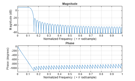
Create a square-root-raised-cosine (SRRC) transmit filter System object™, and then plot the filter response. The results show that the linear filter gain is greater than unity. Specifically, the passband gain is greater than 0 dB.

txfilter = comm.RaisedCosineTransmitFilter;
freqz(txfilter)

Obtain the filter coefficients by using the coeffs object function and adjust the filter gain to unit energy.

b = coeffs(txfilter);

Because a filter with unity passband gain must have filter coefficients that sum to 1, set the linear filter gain to the inverse of the sum of the filter tap coefficients, b.Numerator.

txfilter.Gain = 1/sum(b.Numerator);

Verify that the resulting filter coefficients sum to 1.

bNorm = coeffs(txfilter);
sum(bNorm.Numerator)

ans = 
1.0000

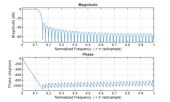
Plot the filter frequency response again. The results now show that the passband gain is 0 dB, which is unity gain.

freqz(txfilter)

Examine Polyphase Matrix of RRC Filter

When you create a multirate filter that uses polyphase decomposition, the polyphase function lets you analyze the component filters individually by returning the components as rows in a matrix. Using polyphase with an output argument returns a matrix containing the polyphase decomposition with individual rows defining each subfilter.

rcfilter = comm.RaisedCosineTransmitFilter;
p = polyphase(rcfilter)

p = 8×11

   -0.0060    0.0097   -0.0133    0.0165   -0.0186    0.3729   -0.0186    0.0165   -0.0133    0.0097   -0.0060
   -0.0051    0.0058   -0.0041   -0.0029    0.0297    0.3621   -0.0524    0.0301   -0.0190    0.0112         0
   -0.0029   -0.0000    0.0075   -0.0255    0.0892    0.3308   -0.0707    0.0368   -0.0206    0.0105         0
    0.0004   -0.0068    0.0196   -0.0477    0.1552    0.2823   -0.0742    0.0364   -0.0184    0.0079         0
    0.0043   -0.0134    0.0300   -0.0653    0.2218    0.2218   -0.0653    0.0300   -0.0134    0.0043         0
    0.0079   -0.0184    0.0364   -0.0742    0.2823    0.1552   -0.0477    0.0196   -0.0068    0.0004         0
    0.0105   -0.0206    0.0368   -0.0707    0.3308    0.0892   -0.0255    0.0075   -0.0000   -0.0029         0
    0.0112   -0.0190    0.0301   -0.0524    0.3621    0.0297   -0.0029   -0.0041    0.0058   -0.0051         0

To analyze the component filters individually, use one of the analysis functions on the corresponding polyphase component vector. For example, to plot the impulse response of the first component filter, use impz on the first vector of the polyphase matrix.

impz(p(1,:))

Extended Capabilities

C/C++ Code Generation

Generate C and C++ code using MATLAB® Coder™.

Usage notes and limitations:

See System Objects in MATLAB Code Generation (MATLAB Coder).

The comm.RaisedCosineTransmitFilter System object supports SIMD code generation using Intel AVX2 technology under these conditions:

• Input signal is real-valued with real filter coefficients.

• Input signal is complex-valued with real or complex filter coefficients.

• Input signal has a data type of single or double.

The SIMD technology significantly improves the performance of the generated code. For details, see Generate SIMD Code from MATLAB Functions for Intel Platforms (Embedded Coder).

Version History

Introduced in R2013b