Viterbi Decoder
Decode convolutionally encoded data using Viterbi algorithm
Libraries:
Communications Toolbox /
Error Detection and Correction /
Convolutional
Communications Toolbox HDL Support /
Error Detection and Correction /
Convolutional
Description
The Viterbi Decoder block decodes convolutionally encoded input symbols to produce binary output symbols by using the Viterbi algorithm. A trellis structure specifies the convolutional encoding scheme. For more information, see Trellis Description of a Convolutional Code.
This block can process several symbols at a time for faster performance and can accept inputs that vary in length during simulation. For more information about variable-size signals, see Variable-Size Signal Basics (Simulink).
This icon shows all the optional block ports enabled.
![]()
Examples
Apply convolutional encoding and BPSK modulation to a binary signal, pass the modulated signal through an AWGN channel. Compute the symbol error rate (SER) of the signal after applying BPSK demodulation and Viterbi decoding.
Explore model
The doc_conv model generates a binary signal by using a Bernoulli Binary Generator block. The Convolutional Encoder block encodes the signal. The BPSK Modulator Baseband block modulates the signal. The AWGN Channel block adds noise to the signal. To demodulate the BPSK modulated signal with zero phase shift, simply extract the value of the real component of the complex symbol demodulation by using the Complex to Real-Imag (Simulink) block. The Viterbi Decoder block decodes the signal. The Error Rate Calculation block computes the SER.

Run simulation
ans =

    'Filtering the signal through an AWGN channel with the EsN0 set to -1 dB, the computed SER is 0.005608.'


ans =

    'For 53499 transmitted symbols, there were 300 symbols errors.'
This example simulates a punctured coding system that uses rate 1/2 convolutional encoding and Viterbi decoding. The complexity of a Viterbi decoder increases rapidly with the code rate. The puncturing technique enables encoding and decoding of higher rate codes by using standard lower rate coders.
The cm_punct_conv_code model transmits a convolutionally encoded BPSK signal through an AWGN channel, demodulates the received signal, and then performs Viterbi decoding to recover the uncoded signal. To compute the error rate, the model compares the original % signal and the decoded signal.

The model uses the PreloadFcn callback function to set these workspace variables for initialization of block parameters:
puncvec = [1;1;0;1;1;0];
EsN0dB = 2;
traceback = 96; % Viterbi traceback depth
For more information, see Model Callbacks (Simulink).
The blocks in this model perform these operations:
Bernoulli Binary Generator — Sets Sample per frames to
3. The block creates a sequence of random bits outputting three samples per frame at each sample time.Convolutional Encoder — Uses the default setting for Trellis structure, selects Puncture code, and sets Puncture vector to the workspace variable
puncvec. The block encodes frames of data by puncturing a rate 1/2, constraint length 7 convolutional code to a rate 3/4 code. The puncture vector specified bypuncvecis the optimal puncture vector for the rate 1/2, constraint length 7 convolutional code. A1in the puncture vector indicates that the bit in the corresponding position of the coded vector is sent to the output vector, while a0indicates that the bit is removed. For the configured encoder, coded bits in positions 1, 2, 4, and 5 are transmitted, while bits in positions 3 and 6 are removed. The rate 3/4 code means that for every 3 bits of input, the punctured code generates 4 bits of output.BPSK Modulator Baseband — Modulates the encoded message using default parameter values.
AWGN Channel — Sets Mode to
Signal to noise ratio (Es/No)and setsEs/No (dB)to the workspace variableEsN0dB. Since the modulator block generates unit power signals, Input signal power, referenced to 1 ohm (watts) keeps its default value of1.Viterbi Decoder — Uses settings for Trellis structure, Punctured code, and Puncture vector that align with the Convolutional Encoder block. The block sets Decision type to
Unquantizedand Traceback depth to thetracebackworkspace variable. To decode the specified convolutional code without puncturing the code, a traceback depth of 40 is sufficient. However, to give the decoder enough data to resolve the ambiguities introduced by the punctures, the block uses a traceback depth of 96 to decode the punctured code. Similar to the convolutional encoder, the puncture vector for the decoder indicates the locations of the punctures. For the decoder, the locations are bits to ignore in the decoding process because the punctured bits are not transmitted and there is no information to indicate their values. Each 1 in the puncture vector indicates a transmitted bit, and each 0 indicates a punctured bit to ignore in the input to the decoder.Complex to Real-Imag (Simulink) — Demodulates the BPSK signal by extracting the real part of the complex samples.
Error Rate Calculation — Uses the Receive delay value to account for total number of samples of system delay and compares the decoded bits to the original source bits. The block outputs a three-element vector containing the calculated BER, the number of errors observed, and the number of bits processed. The Receive delay is set to the
tracebackworkspace variable because the Viterbi traceback depth causes the only delay in the system. Typically, BER simulations run until a minimum number of errors have occurred, or until the simulation processes a maximum number of bits. The Error Rate Calculation block selects the Stop simulation parameter and sets the target number of errors to100and the maximum number of symbols to1e6to control the duration of the simulation.
Evaluate Bit Error Rate
Generate a bit error rate curve by running this code to simulate the model over a range of EbN0 settings.
Compare the simulation results with an approximation of the bit error probability bound for a punctured code as per [ 1 ]. The bit error rate performance of a rate  punctured code is bounded above by the expression:

In this expression, erfc denotes the complementary error function,  is the code rate, and both
  and
and  are dependent on the particular code. For the rate 3/4 code of this example, = 5,
  = 42,
= 42,  = 201,
  = 1492, and so on. For more information, see reference [ 1 ].
Compute an approximation of the theoretical bound using the first seven terms of the summation for Eb/N0 values in 2:0.02:5. The values used for nerr come from reference [ 2 ], Table II.
Plot the simulation results, a fitted curve, and theoretical bounds.

In some cases, at the lower bit error rates, you might notice simulation results that appear to indicate error rates slightly above the bound. This result can come from the finite traceback depth in the decoder or, if you observe fewer than 500 bit errors, from simulation variance.
For an example that shows convolutional coding without puncturing, see the Soft-Decision Decoding section in Error Detection and Correction.
References
Yasuda, Y., K. Kashiki, and Y. Hirata, "High Rate Punctured Convolutional Codes for Soft Decision Viterbi Decoding," IEEE Transactions on Communications, Vol. COM-32, March, 1984, pp. 315–319.
Begin, G., Haccoun, D., and Paquin, C., "Further results on High-Rate Punctured Convolutional Codes for Viterbi and Sequential Decoding," IEEE Transactions on Communications, Vol. 38, No. 11, November, 1990, p. 1923.
Use the Viterbi Decoder block for fixed-point hard- and soft-decision convolutional decoding. Compare results to theoretical upper bounds as computed with the Bit Error Rate Analysis app.
Simulation Configuration
The cm_viterbi_harddec_fixpt and cm_viterbi_softdec_fixpt models highlight the fixed-point modeling attributes of the Viterbi decoder, using similar layouts. The default configuration of the models use the PreLoadFcn Callback to specify an  setting of 4 dB for the AWGN Channel block. The convolutional encoder is configured as a rate 1/2 encoder. Specifically, for every 2 bits the encoder adds another 2 redundant bits. To accommodate the code rate, the Eb/No (dB) parameter of the AWGN block is halved by subtracting
 10*log10(2) from the assigned setting. To limit the run duration to 100 errors or 1e6 bits for the Error Rate Calculation block.
Fixed-Point Modeling
Fixed-point modeling enables bit-true simulations which take into account hardware implementation considerations and the dynamic range of the data and parameters. For example, if the target hardware is a DSP microprocessor, some of the possible word lengths are 8, 16, or 32 bits, whereas if the target hardware is an ASIC or FPGA, there may be more flexibility in the word length selection.
To enable fixed-point Viterbi decoding,
For hard decisions, the block input must be of type ufix1 (unsigned integer of word length 1). Based on this input (either a 0 or a 1), the internal branch metrics are calculated using an unsigned integer of word length = (number of output bits), as specified by the trellis structure (which equals 2 for the hard-decision example).
For soft decisions, the block input must be of type ufixN (unsigned integer of word length N), where N is the number of soft-decision bits, to enable fixed-point decoding. The block inputs must be integers in the range 0 to
 . The internal branch metrics are calculated using an unsigned integer of word length = (N + number of output bits - 1), as specified by the trellis structure (which equals 4 for the soft-decision example).
The State metric word length is specified by the user and usually must be greater than the branch metric word length already calculated. You can tune this to be the most suitable value (based on hardware and data considerations) by reviewing the logged data for the system.
Enable the logging by selecting Apps > Fixed-Point Tool. In the Fixed-Point Setting menu, set the Fixed-point instruments mode to Minimums, maximums and overflows, and rerun the simulation. If you see overflows, it implies the data did not fit in the selected container. You could either try scaling the data prior to processing it or, if your hardware allows, increase the size of the word length. Based on the minimum and maximum values of the data, you are also able to determine whether the selected container is of the appropriate size.
Try running simulations with different values of State metric word length to get an idea of its effect on the algorithm. You should be able to narrow down the parameter to a suitable value that has no adverse effect on the BER results.
The hard decision configuration for the cm_viterbi_harddec_fixpt model:

The BPSK Demodulator Baseband produces hard decisions, which are passed onto the decoder.
The Data Type Conversion (Simulink) block sets the
Modeparameter toFixed pointand casts the output data type tofixdt(0,1,0). The signal input to the Viterbi Decoder block isufix1.
The Viterbi Decoder block has the
Decision typeparameter set toHard decision, and on the Data Types tab, theState metric word lengthis set to4and theOutput data typeis set toboolean. The bit error rate is displayed and captured to theBERworkspace variable.
The soft decision configuration for the cm_viterbi_softdec_fixpt model:
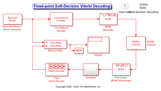
The BPSK Demodulator Baseband produces soft decisions using the log-likelihood ratio. These soft outputs are 3-bit quantized and passed onto the decoder.
A Quantizer subsystem (containing Gain (Simulink), Scalar Quantizer Encoder, and Data Type Conversion (Simulink) blocks) quantizes the signal and casts the output data type to
fixdt(0,3,0). The signal input to the Viterbi Decoder block isufix3.
The Viterbi Decoder block has the
Decision typeparameter set toSoft decisionandNumber of soft decision bitsset to 3, and on the Data Types tab, theState metric word lengthis set to6and theOutput data typeis set toboolean. The bit error rate is displayed and captured to theBERworkspace variable.
Comparisons Between Hard and Soft-Decision Decoding
The two models are configured to run from within the Bit Error Rate Analysis app to generate simulation curves to compare the BER performance for hard-decision versus soft-decision decoding.
You can produce the results in this plot by following the steps outlined below.
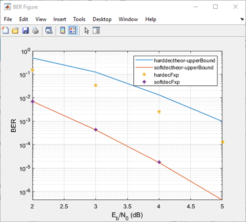
These steps generate simulation results for theoretical and fixed-point hard and soft decision Viterbi decoding:
Open the Bit Error Rate Analysis app by selecting it in the Apps tab or by entering
bertoolat the MATLAB command prompt.On the Theoretical pane, with Eb/N0 range set to 2:5, Channel type set to
AWGN, Modulation type set toPSK, Channel coding set toConvolutional, run with Decision method set toHardand thenSoft. Rename the BER Data Set to identify the hard and soft data sets of theoretical results.On the Monte Carlo pane, set Eb/N0 range to 2:1:5, for Simulation environment select
Simulink, BER variable name set toBER, for Simulation limits set Number of errors to 100 and Number of bits to 1e6. Run with Model name set tocm_viterbi_harddec_fixptand thencm_viterbi_softdec_fixpt. Rename the BER Data Set to identify the hard and soft data sets of Simulink results.
After the four runs the app will resemble this image.

Comparisons with Double-Precision Data
For further explorations, you can run the same model with double precision data by selecting Apps > Fixed-Point Tool. In the Fixed-Point Tool app, select the Data type override to be Double. This selection overrides all data type settings in all the blocks to use double precision. For the Viterbi Decoder block, as Output type was set to boolean, this parameter should also be set to double.
Upon simulating the model, note that the double-precision and fixed-point BER results are the same. They are the same because the fixed-point parameters for the model have been selected to avoid any loss of precision and optimize memory efficiency.
Extended Examples

Tail-Biting Convolutional Coding
Use the Convolutional Encoder and Viterbi Decoder blocks to simulate a tail-biting convolutional code.
Ports
Input
Output
Parameters
Block Characteristics
More About
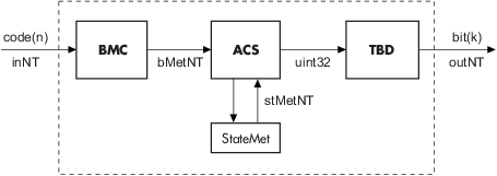
There are three main components to the Viterbi decoding algorithm. They are branch metric computation (BMC), add-compare and select (ACS), and traceback decoding (TBD). This diagram illustrates the signal flow for a k/n rate code.
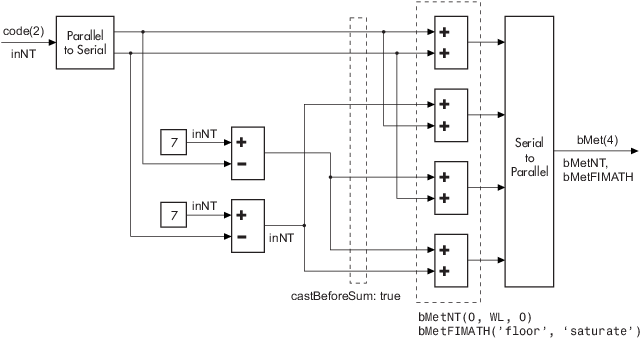
This diagram illustrates the BMC for a 1/2 rate, nsdec = 3 signal flow.
This diagram illustrates an ACS component cycle, where
WL2 is specified on the mask by the user.
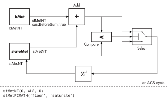
In these flow diagrams, inNT, bMetNT , stMetNT, and outNT are numerictype (Fixed-Point Designer) objects, and bMetFIMATH and
stMetFIMATH, are fimath (Fixed-Point Designer)
objects.
References
[1] Clark, George C., and J. Bibb Cain. Error-Correction Coding for Digital Communications. Applications of Communications Theory. New York: Plenum Press, 1981.
[2] Gitlin, Richard D., Jeremiah F. Hayes, and Stephen B. Weinstein. Data Communications Principles. Applications of Communications Theory. New York: Plenum Press, 1992.
[3] Heller, J., and I. Jacobs. “Viterbi Decoding for Satellite and Space Communication.” IEEE® Transactions on Communication Technology 19, no. 5 (October 1971): 835–48. https://doi.org/10.1109/TCOM.1971.1090711.
[4] Yasuda, Y., K. Kashiki, and Y. Hirata. “High-Rate Punctured Convolutional Codes for Soft Decision Viterbi Decoding.” IEEE Transactions on Communications 32, no. 3 (March 1984): 315–19. https://doi.org/10.1109/TCOM.1984.1096047.
[5] Haccoun, D., and G. Begin. “High-Rate Punctured Convolutional Codes for Viterbi and Sequential Decoding.” IEEE Transactions on Communications 37, no. 11 (November 1989): 1113–25. https://doi.org/10.1109/26.46505.
[6] Begin, G., D. Haccoun, and C. Paquin. “Further Results on High-Rate Punctured Convolutional Codes for Viterbi and Sequential Decoding.” IEEE Transactions on Communications 38, no. 11 (November 1990): 1922–28. https://doi.org/10.1109/26.61470.
[7] Moision, B. "A Truncation Depth Rule of Thumb for Convolutional Codes." In Information Theory and Applications Workshop (January 27 2008-February 1 2008, San Diego, California), 555-557. New York: IEEE, 2008.