S-Parameter Import, Plotting, and Writing | Getting Started with S-Parameters, Part 1
From the series: Getting Started with S-Parameters
Learn how to import Touchstone data files into MATLAB® and access network data such as S-parameters. See how to inspect S-parameter data, select an arbitrary frequency range, and plot the magnitude and phase responses on a Smith chart. Find out how to save n-port Touchstone files.
Published: 7 Oct 2021
Welcome to this first part of The MathWorks webinar technical series regarding S-parameter analysis using MATLAB. In this installment, basic s-parameter analysis is performed where S-parameter data is imported and plotted on both rectangular and polar plots. Finally, you will be shown how to write S-parameter data to a touchstone data file.
Let's begin by getting familiar with the functions that are going to be used today. Namely, S-parameters, rfplot, smith, and rfwrite. Help for each of these RF toolbox functions can be found by typing in Help and the function name at the MATLAB command prompt, or typing in the function name in the Help browser. Remembering all the various MATLAB function names can be burdensome. And I recommend that instead of memorizing all the names, that you refer to product examples to recall the use of these functions.
A couple of RF toolbox examples that I would recommend include the following.
First, modeling a high-speed backplane. This example readily shows the user how to import as parameters into MATLAB, manipulate the various as parameter objects, and finally, how to easily plot the S-parameter response on a rectangular plot.
Second, writing the touchstone file. This second example is a good reference example for saving S-parameter data into a multi port touchstone data file, and provides a workflow example that can be easily followed.
Now let's go through an example of doing all of this. First, let us import the data from a 4 port S-parameter data file and assign it to a MATLAB data object. Let's call it s4p. Type in s4p = sparameters default .s4p.
Notice that there are properties for frequency, impedance, the S-parameters, and the number of ports that the file has. Let's now plot the magnitude response for elements 1,1 and 2,1 of this S-parameter object.
First, open a new figure. Then use the RF plot function that calls the S-parameter object as well as the matrix element that is to be plotted. To plot on the same figure, invoke the Hold command, and then plot the next S-parameter element that you want to visualize.
To view the phase response, the process is very similar, except you need to add the plot flag angle into the RF plot to view this figure. Start by opening a new figure, use the RF plot function, but add the Angle plot flag, and finally turn on the grid.
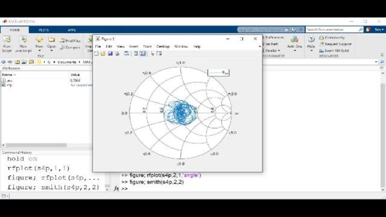
In a similar fashion, diagonal elements at the S-parameter data can be plotted on a Smith chart. To do this, use the Smith function. Again, let's add a new figure, and then plot the response of element 2,2.
For the final part of today's session, let's create a new S-parameter data file that only contains the data of s4p to 10 gigahertz. The process to do this from the MATLAB command window is straightforward.
First, assign a file name of your new S-parameter file to a MATLAB variable. Let's use filename = new_s4p_data.s4p.
Next, you will need to determine the frequency vector index value that corresponds to 10 gigahertz. This is done by using the Find function.
Next, you would use the RF Write function in the following manner. First, call the S-parameter data to be written to the new data file. Then, call the frequency range associated with the data and then include the file name. Once executed, you can see the new data file has been saved to my working directory.
I hope that you have found this video useful. And next time we will be looking at using MATLAB for concatenating arbitrary S parameter data sets together.


