Visualize and Recreate TQWT Decomposition
This example shows how to visualize a tunable Q-factor wavelet transform (TQWT) decomposition using Signal Multiresolution Analyzer. You learn how to compare two different decompositions in the app, and how to recreate a decomposition in your workspace.
Load an ECG signal.
load wecgVisualize TQWT
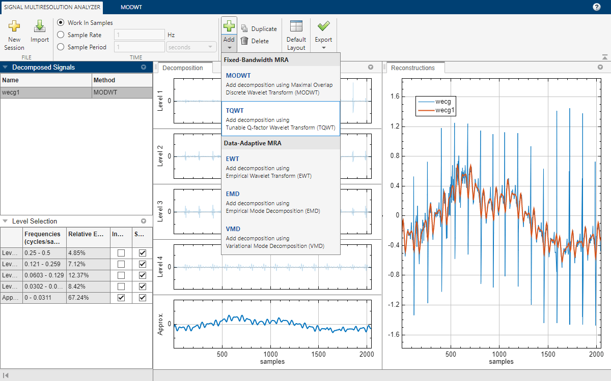
Open Signal Multiresolution Analyzer and click Import. Select the ECG signal and click Import. By default, a four-level MODWTMRA decomposition appears in the MODWT tab.
To generate an MRA decomposition using the tunable Q-factor wavelet transform (TQWT), go to the Signal Multiresolution Analyzer tab. Click Add ▼ and select TQWT.
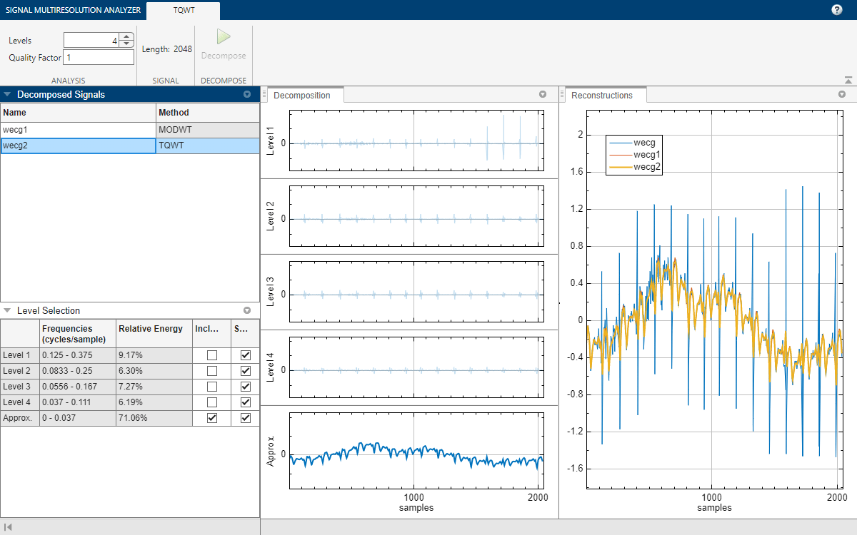
After a few moments, the TQWT decomposition wecg2 appears in the TQWT tab. The app obtains the decomposition using the tqwt and tqwtmra functions with default settings. You can change the level of decomposition and TQWT quality factor using the toolstrip. Changing a value enables the Decompose button.
The Level Selection pane shows the relative energies of the signal across scales, as well as the theoretical frequency ranges. The ranges are derived from the center frequencies and approximate bandwidths of the wavelet subbands, as defined by Selesnick [1]. For more information, see Tunable Q-factor Wavelet Transform.
Adjust Q-factor
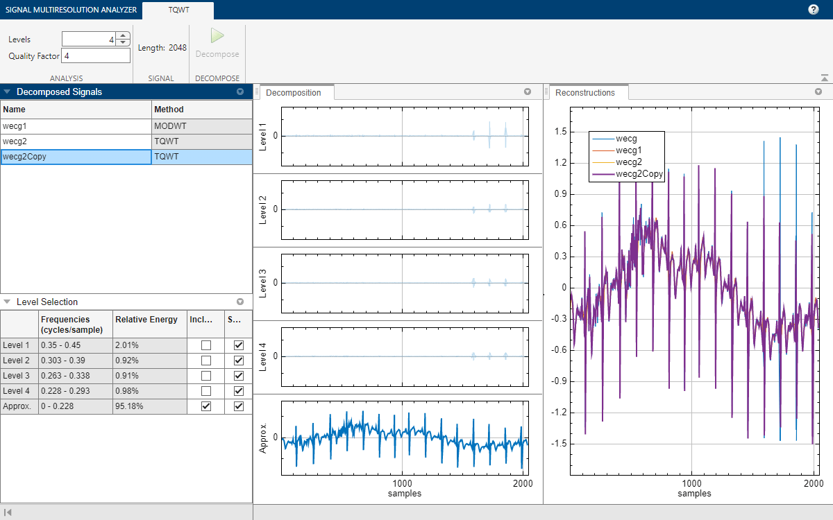
According to the Level Selection pane, the approximation contains 71% of the total signal energy. To investigate the impact of the quality factor on the approximation, first select wecg2 and click Duplicate on the Signal Multiresolution Analyzer tab. The decomposition wecg2Copy appears. On the TQWT tab, enter a quality factor value of 4 and click Decompose. The relative energy in the resulting approximation has increased to 95%.
Export Script
To recreate the decomposition in your workspace, in the Signal Multiresolution Analyzer tab click Export > Generate MATLAB Script. An untitled script opens in your editor with the following executable code. The true-false values in levelForReconstruction correspond to the Include boxes you selected in the Level Selection pane. You can save the script as is or modify it to apply the same decomposition settings to other signals. Run the code.
% Logical array for selecting reconstruction elements
levelForReconstruction = [false,false,false,false,true];

% Perform the decomposition using tqwt
[wt,info] = tqwt(wecg, ...
    Level=4, ...
    QualityFactor=4);

% Construct MRA matrix using tqwtmra
mra = tqwtmra(wt, 2048, QualityFactor=4);

% Sum down the rows of the selected multiresolution signals
wecg2Copy = sum(mra(levelForReconstruction,:),1);
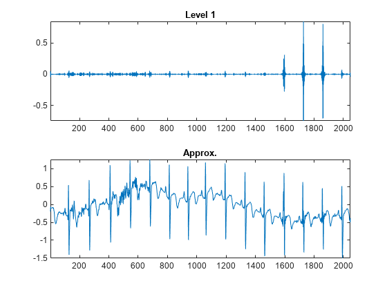
The rows in the MRA matrix mra correspond to the levels and approximation in the Level Selection pane. Plot the first and last rows in mra. Confirm the plots are identical to the first level plot and the approximation plot in the Decomposition pane.
tiledlayout(2,1)
nexttile
plot(mra(1,:))
axis tight
title("Level 1")
nexttile
plot(mra(end,:))
title("Approx.")
axis tight
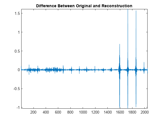
To compare the reconstruction, which consists of only the approximation, with the original signal, plot the difference between the two.
figure
plot(wecg-wecg2Copy')
axis tight
title("Difference Between Original and Reconstruction")
References
[1] Selesnick, Ivan W. “Wavelet Transform With Tunable Q-Factor.” IEEE Transactions on Signal Processing 59, no. 8 (August 2011): 3560–75. https://doi.org/10.1109/TSP.2011.2143711.