Least Asymmetric Wavelet and Phase
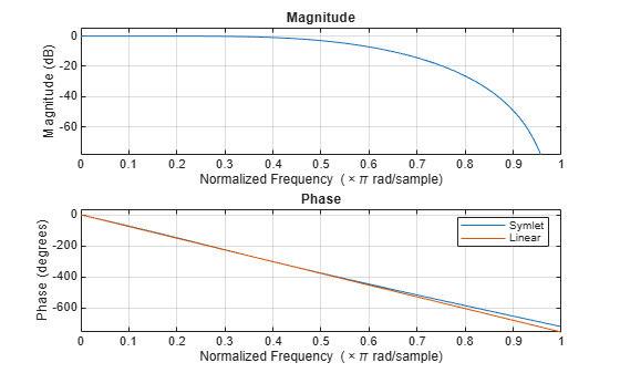
Obtain the scaling filter associated with the symlet of order 4.
n = 4;
scal_sym = daubfactors(n,"sym");
Use the function freqz (Signal Processing Toolbox) to plot the frequency response of the filter. Compare the phase angle with a linear phase filter.
freqz(scal_sym)
subPlots = get(gcf,"Children");
phasePlot = subPlots(2);
yLimits = get(phasePlot,"Ylim");
hold(phasePlot,"on");
plot(phasePlot,[0 1],[0 yLimits(1)])
legend(phasePlot,"Symlet","Linear")
hold(phasePlot,"off")
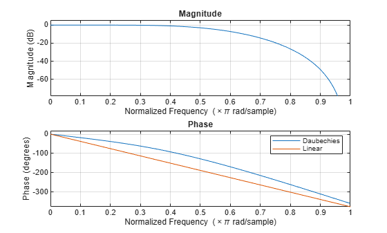
Obtain the scaling filter associated with the Daubechies wavelet of order 4. Plot the frequency response of the filter. Compare the phase angle with a linear phase filter.
db_sym = daubfactors(n);

freqz(db_sym)
subPlots = get(gcf,"Children");
phasePlot = subPlots(2);
yLimits = get(phasePlot,"Ylim");
hold(phasePlot,"on");
plot(phasePlot,[0 1],[0 yLimits(1)])
legend(phasePlot,"Daubechies","Linear")
hold(phasePlot,"off")