symaux

Symlet wavelet filter computation

Syntax

w = symaux(n)

w = symaux(___,sumw)

Description

The symaux function generates the scaling filter coefficients for the "least asymmetric" Daubechies wavelets.

w = symaux(n) is the order n Symlet scaling filter such that sum(w) = 1.

Note

• Instability may occur when n is too large. Starting with values of n in the 30s range, function output will no longer accurately represent scaling filter coefficients.

• As n increases, the time required to compute the filter coefficients rapidly grows.

• For n = 1, 2, and 3, the order n Symlet filters and order n Daubechies filters are identical. See Extremal Phase Wavelet.

w = symaux(___,sumw) is the order n Symlet scaling filter such that sum(w) = sumw.

w = symaux(n,0) is equivalent to w = symaux(n,1).

Examples

Unit Norm Scaling Filter Coefficients

In this example you will generate symlet scaling filter coefficients whose norm is equal to 1. You will also confirm the coefficients satisfy a necessary relation.

Compute the scaling filter coefficients of the order 10 symlet whose sum equals$\sqrt{2}$.

n = 10;
w = symaux(n,sqrt(2));

Confirm the sum of the coefficients is equal to $\sqrt{2}$ and the norm is equal to 1.

sqrt(2)-sum(w)

ans = 
2.2204e-16

1-sum(w.^2)

ans = 
-3.3307e-14

Since integer translations of the scaling function form an orthogonal basis, the coefficients satisfy the relation ${\sum }_{\mathit{n}}\mathit{w}\left(\mathit{n}\right)\mathit{w}\left(\mathit{n}-2\mathit{k}\right)=\delta \left(\mathit{k}\right)$. Confirm this by taking the autocorrelation of the coefficients and plotting the result.

corrw = xcorr(w,w);
stem(corrw)
grid on
title('Autocorrelation of scaling coefficients')

stem(corrw(2:2:end))
grid on
title('Even-indexed autocorrelation values')

Symlet and Daubechies Scaling Filters

This example shows that symlet and Daubechies scaling filters of the same order are both solutions of the same polynomial equation.

Generate the order 4 Daubechies scaling filter and plot it.

wdb4 = dbaux(4);
stem(wdb4)
title('Order 4 Daubechies Scaling Filter')

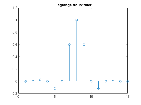
wdb4 is a solution of the equation: P = conv(wrev(w),w)*2, where P is the "Lagrange trous" filter for N = 4. Evaluate P and plot it. P is a symmetric filter and wdb4 is a minimum phase solution of the previous equation based on the roots of P.

P = conv(wrev(wdb4),wdb4)*2;
stem(P)
title('''Lagrange trous'' filter')

Generate wsym4, the order 4 symlet scaling filter and plot it. The Symlets are the "least asymmetric" Daubechies' wavelets obtained from another choice between the roots of P.

wsym4 = symaux(4);
stem(wsym4)
title('Order 4 Symlet Scaling Filter')

Compute conv(wrev(wsym4),wsym4)*2 and confirm that wsym4 is another solution of the equation P = conv(wrev(w),w)*2.

P_sym = conv(wrev(wsym4),wsym4)*2;
err = norm(P_sym-P)

err = 
1.2491e-15

Least Asymmetric Wavelet and Phase

For a given support, the orthogonal wavelet with a phase response that most closely resembles a linear phase filter is called least asymmetric. Symlets are examples of least asymmetric wavelets. They are modified versions of the classic Daubechies db wavelets. In this example, you will show that the order 4 symlet has a nearly linear phase response, while the order 4 Daubechies wavelet does not.

First plot the order 4 symlet and order 4 Daubechies scaling functions. While neither is perfectly symmetric, note how much more symmetric the symlet is.

[phi_sym,~,xval_sym]=wavefun('sym4',10);
[phi_db,~,xval_db]=wavefun('db4',10);
subplot(2,1,1)
plot(xval_sym,phi_sym)
title('sym4 - Scaling Function')
grid on
subplot(2,1,2)
plot(xval_db,phi_db)
title('db4 - Scaling Function')
grid on

Generate the filters associated with the order 4 symlet and Daubechies wavelets.

scal_sym = symaux(4,sqrt(2));
scal_db = dbaux(4,sqrt(2));

Compute the frequency response of the scaling synthesis filters.

[h_sym,w_sym] = freqz(scal_sym);
[h_db,w_db] = freqz(scal_db);

To avoid visual discontinuities, unwrap the phase angles of the frequency responses and plot them. Note how well the phase angle of the symlet filter approximates a straight line.

h_sym_u = unwrap(angle(h_sym));
h_db_u = unwrap(angle(h_db));
figure
plot(w_sym/pi,h_sym_u,'.')
hold on
plot(w_sym([1 end])/pi,h_sym_u([1 end]),'r')
hold off
grid on
xlabel('Normalized Frequency ( x \pi rad/sample)')
ylabel('Phase (radians)')
legend('Phase Angle of Frequency Response','Straight Line')
title('Symlet Order 4 - Phase Angle')

figure
plot(w_db/pi,h_db_u,'.')
hold on
plot(w_db([1 end])/pi,h_db_u([1 end]),'r')
hold off
grid on
xlabel('Normalized Frequency ( x \pi rad/sample)')
ylabel('Phase (radians)')
legend('Phase Angle of Frequency Response','Straight Line')
title('Daubechies Order 4 - Phase Angle')

The sym4 and db4 wavelets are not symmetric, but the biorthogonal wavelet is. Plot the scaling function associated with the bior3.5 wavelet. Compute the frequency response of the synthesis scaling filter for the wavelet and verify that it has linear phase.

[~,~,phi_bior_r,~,xval_bior]=wavefun('bior3.5',10);
figure
plot(xval_bior,phi_bior_r)
title('bior3.5 - Scaling Function')
grid on

[LoD_bior,HiD_bior,LoR_bior,HiR_bior] = wfilters('bior3.5');
[h_bior,w_bior] = freqz(LoR_bior);
h_bior_u = unwrap(angle(h_bior));
figure
plot(w_bior/pi,h_bior_u,'.')
hold on
plot(w_bior([1 end])/pi,h_bior_u([1 end]),'r')
hold off
grid on
xlabel('Normalized Frequency ( x \pi rad/sample)')
ylabel('Phase (radians)')
legend('Phase Angle of Frequency Response','Straight Line')
title('Biorthogonal 3.5 - Phase Angle')

Demonstrate Extremal Phase Property

This example demonstrates that for a given support, the cumulative sum of the squared coefficients of a scaling filter increase more rapidly for an extremal phase wavelet than other wavelets.

Generate the scaling filter coefficients for the db15 and sym15 wavelets. Both wavelets have support of width $2\times 15-1=29$.

[~,~,LoR_db,~] = wfilters('db15');
[~,~,LoR_sym,~] = wfilters('sym15');

Next, generate the scaling filter coefficients for the coif5 wavelet. This wavelet also has support of width $6\times 5-1=29$.

[~,~,LoR_coif,~] = wfilters('coif5');

Confirm the sum of the coefficients for all three wavelets equals $\sqrt{2}$.

sqrt(2)-sum(LoR_db)

ans = 
4.4409e-16

sqrt(2)-sum(LoR_sym)

ans = 
-2.2204e-16

sqrt(2)-sum(LoR_coif)

ans = 
2.2204e-16

Plot the cumulative sums of the squared coefficients. Note how rapidly the Daubechies sum increases. This is because its energy is concentrated at small abscissas. Since the Daubechies wavelet has extremal phase, the cumulative sum of its squared coefficients increases more rapidly than the other two wavelets.

plot(cumsum(LoR_db.^2),'rx-')
hold on
plot(cumsum(LoR_sym.^2),'mo-')
plot(cumsum(LoR_coif.^2),'b*-')
hold off
legend('Daubechies','Symlet','Coiflet')
title('Cumulative Sum')

Input Arguments

n — Order of symlet

positive integer

Order of the symlet, specified as a positive integer.

sumw — Sum of coefficients

1 (default) | positive real number

Sum of the scaling filter coefficients, specified as a positive real number. Set to sqrt(2) to generate vector of coefficients whose norm is 1.

Output Arguments

w — Filter coefficients

row vector

Vector of scaling filter coefficients of the order n symlet.

The scaling filter coefficients satisfy a number of properties. You can use these properties to check your results. See Unit Norm Scaling Filter Coefficients for additional information.

More About

Least Asymmetric Wavelet

The Haar wavelet, also known as the Daubechies wavelet of order 1, db1, is the only compactly supported orthogonal wavelet that is symmetric, or equivalently has linear phase. No other compactly supported orthogonal wavelet can be symmetric. However, it is possible to derive wavelets which are minimally asymmetric, meaning that their phase will be very nearly linear. For a given support, the orthogonal wavelet with a phase response that most closely resembles a linear phase filter is called least asymmetric.

Extremal Phase Wavelet

Constructing a compactly supported orthogonal wavelet basis involves choosing roots of a particular polynomial equation. Different choices of roots will result in wavelets whose phases are different. Choosing roots that lie within the unit circle in the complex plane results in a filter with highly nonlinear phase. Such a wavelet is said to have extremal phase, and has energy concentrated at small abscissas. Let {h_k} denote the set of scaling coefficients associated with an extremal phase wavelet, where k = 1,…,M. Then for any other set of scaling coefficients {g_k} resulting from a different choice of roots, the following inequality holds for all J = 1,…,M:

$${\displaystyle \sum _{k=1}^J{g}_k^2\le }{\displaystyle \sum _{k=1}^J{h}_k^2}.$$

The {h_k} are sometimes called a minimal delay filter [2].

The polynomial equation mentioned above depends on the desired number of vanishing moments N for the wavelet. To construct a wavelet basis involves choosing roots of the equation. In the case of least asymmetric wavelets and extremal phase wavelets for orders 1, 2, and 3, there are effectively no choices to make. For N = 1, 2, and 3, the dbN and symN filters are equal. The example Symlet and Daubechies Scaling Filters shows that two different scaling filters can satisfy the same polynomial equation. For additional information, see Daubechies [1].

References

[1] Daubechies, I. Ten Lectures on Wavelets, CBMS-NSF Regional Conference Series in Applied Mathematics. Philadelphia, PA: SIAM Ed, 1992.

[2] Oppenheim, Alan V., and Ronald W. Schafer. Discrete-Time Signal Processing. Englewood Cliffs, NJ: Prentice Hall, 1989.

Version History

Introduced before R2006a