dbaux

(To be removed) Daubechies wavelet filter computation

dbaux will be removed in a future release. Use daubfactors instead. (since R2026a) For more information, see Version History.

Syntax

W = dbaux(N)

W = dbaux(N,SUMW)

Description

The dbaux function generates the scaling filter coefficients for the "extremal phase" Daubechies wavelets.

W = dbaux(N) is the order N Daubechies scaling filter such that sum(W) = 1.

Note

• Instability might occur when N is too large. Starting with values of N in the 30s range, function output will no longer accurately represent scaling filter coefficients.

• For N = 1, 2, and 3, the order N Symlet filters and order N Daubechies filters are identical. See Extremal Phase Wavelet.

W = dbaux(N,SUMW) is the order N Daubechies scaling filter such that sum(W) = SUMW.

W = dbaux(N,0) is equivalent to W = dbaux(N,1).

Examples

Daubechies Extremal Phase Scaling Filter with Specified Sum

This example shows how to determine the Daubechies extremal phase scaling filter with a specified sum. The two most common values for the sum are $$\sqrt{2}$$ and 1.

Construct two versions of the db4 scaling filter. One scaling filter sums to $$\sqrt{2}$$ and the other version sums to 1.

NumVanishingMoments = 4;
h = dbaux(NumVanishingMoments,sqrt(2));
m0 = dbaux(NumVanishingMoments,1);

The filter with sum equal to $$\sqrt{2}$$ is the synthesis (reconstruction) filter returned by wfilters and used in the discrete wavelet transform.

[LoD,HiD,LoR,HiR] = wfilters('db4');
max(abs(LoR-h))

ans = 
4.2614e-13

For orthogonal wavelets, the analysis (decomposition) filter is the time-reverse of the synthesis filter.

max(abs(LoD-fliplr(h)))

ans = 
4.2614e-13

Symlet and Daubechies Scaling Filters

This example shows that symlet and Daubechies scaling filters of the same order are both solutions of the same polynomial equation.

Generate the order 4 Daubechies scaling filter and plot it.

wdb4 = dbaux(4);
stem(wdb4)
title('Order 4 Daubechies Scaling Filter')

wdb4 is a solution of the equation: P = conv(wrev(w),w)*2, where P is the "Lagrange trous" filter for N = 4. Evaluate P and plot it. P is a symmetric filter and wdb4 is a minimum phase solution of the previous equation based on the roots of P.

P = conv(wrev(wdb4),wdb4)*2;
stem(P)
title('''Lagrange trous'' filter')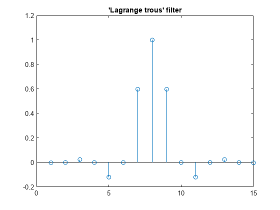

Generate wsym4, the order 4 symlet scaling filter and plot it. The Symlets are the "least asymmetric" Daubechies' wavelets obtained from another choice between the roots of P.

wsym4 = symaux(4);
stem(wsym4)
title('Order 4 Symlet Scaling Filter')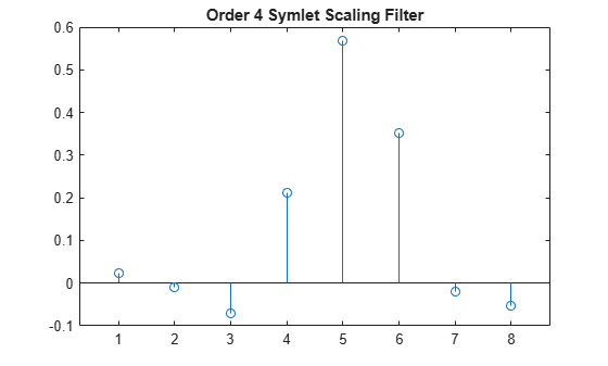

Compute conv(wrev(wsym4),wsym4)*2 and confirm that wsym4 is another solution of the equation P = conv(wrev(w),w)*2.

P_sym = conv(wrev(wsym4),wsym4)*2;
err = norm(P_sym-P)

err = 
1.2491e-15

Input Arguments

N — Order of Daubechies scaling filter

positive integer

Order of Daubechies scaling filter, specified as a positive integer.

Data Types: single | double

SUMW — Sum of coefficients

1 (default) | positive scalar

Sum of coefficients, specified as a positive scalar. Set to sqrt(2) to generate vector of coefficients whose norm is 1.

Data Types: single | double

Output Arguments

W — Scaling filter coefficients

vector

Scaling filter coefficients returned as a vector.

The scaling filter coefficients satisfy a number of properties. As the example Daubechies Extremal Phase Scaling Filter with Specified Sum demonstrates, you can construct scaling filter coefficients with a specific sum. If {h_k} denotes the set of order N Daubechies scaling filter coefficients, where n = 1, ..., 2N, then $${\displaystyle \sum _{n=1}^{2N}{h}_n^2=1.}$$ The coefficients also satisfy the relation $${\displaystyle {\sum }_{n}h(n)h(n-2k)=\delta (k).}$$ You can use these properties to check your results.

Limitations

• The computation of the dbN Daubechies scaling filter requires the extraction of the roots of a polynomial of order 4N. Instability may occur beginning with values of N in the 30s.

More About

Extremal Phase Wavelet

Constructing a compactly supported orthogonal wavelet basis involves choosing roots of a particular polynomial equation. Different choices of roots will result in wavelets whose phases are different. Choosing roots that lie within the unit circle in the complex plane results in a filter with highly nonlinear phase. Such a wavelet is said to have extremal phase, and has energy concentrated at small abscissas. Let {h_k} denote the set of scaling coefficients associated with an extremal phase wavelet, where k = 1,…,M. Then for any other set of scaling coefficients {g_k} resulting from a different choice of roots, the following inequality holds for all J = 1,…,M:

$${\displaystyle \sum _{k=1}^J{g}_k^2\le }{\displaystyle \sum _{k=1}^J{h}_k^2}.$$

The {h_k} are sometimes called a minimal delay filter [2].

The polynomial equation mentioned above depends on the number of vanishing moments N for the wavelet. To construct a wavelet basis involves choosing roots of the equation. In the case of least asymmetric wavelets and extremal phase wavelets for orders 1, 2, and 3, there are effectively no choices to make. For N = 1, 2, and 3, the dbN and symN filters are equal. The example Symlet and Daubechies Scaling Filters shows that two different scaling filters can satisfy the same polynomial equation. For additional information, see Daubechies [1].

Least Asymmetric Wavelet

The Haar wavelet, also known as the Daubechies wavelet of order 1, db1, is the only compactly supported orthogonal wavelet that is symmetric, or equivalently has linear phase. No other compactly supported orthogonal wavelet can be symmetric. However, it is possible to derive wavelets which are minimally asymmetric, meaning that their phase will be very nearly linear. For a given support, the orthogonal wavelet with a phase response that most closely resembles a linear phase filter is called least asymmetric.

Algorithms

The algorithm used is based on a result obtained by Shensa [3], showing a correspondence between the “Lagrange à trous” filters and the convolutional squares of the Daubechies wavelet filters.

The computation of the order N Daubechies scaling filter w proceeds in two steps: compute a “Lagrange à trous” filter P, and extract a square root. More precisely:

• P the associated “Lagrange à trous” filter is a symmetric filter of length 4N-1. P is defined by

  P = [a(N) 0 a(N-1) 0 ... 0 a(1) 1 a(1) 0 a(2) 0 ... 0 a(N)]

• where

  

• Then, if w denotes dbN Daubechies scaling filter of sum , w is a square root of P:

      P = conv(wrev(w),w) where w is a filter of length 2N.

  The corresponding polynomial has N zeros located at −1 and N−1 zeros less than 1 in modulus.

Note that other methods can be used; see various solutions of the spectral factorization problem in Strang-Nguyen [4] (p. 157).

References

[1] Daubechies, I. Ten Lectures on Wavelets, CBMS-NSF Regional Conference Series in Applied Mathematics. Philadelphia, PA: SIAM Ed, 1992.

[2] Oppenheim, Alan V., and Ronald W. Schafer. Discrete-Time Signal Processing. Englewood Cliffs, NJ: Prentice Hall, 1989.

[3] Shensa, M.J. (1992), “The discrete wavelet transform: wedding the a trous and Mallat Algorithms,” IEEE Trans. on Signal Processing, vol. 40, 10, pp. 2464-2482.

[4] Strang, G., and T. Nguyen.Wavelets and Filter Banks. Wellesley, MA: Wellesley-Cambridge Press, 1996.

Version History

Introduced before R2006a

R2026a: To be removed

dbaux runs without warning but will be removed in a future release. Use daubfactors instead.. The function unifies the functionality of dbaux and symaux, as well, enabling you to obtain the scaling filters of the three Daubechies families, "csym", "db", and "sym", through a single interface.