Boundary Effects in Real-Valued Bandlimited Shearlet Systems
This example shows how edge effects can result in shearlet coefficients with nonzero imaginary parts even in a real-valued shearlet system. The example also discusses two strategies for mitigating these boundary effects: resizing or padding the image and changing the number of scales.
The bandlimited cone-adapted finite shearlet transform implemented in the shearletSystem object is developed in [1] and [2]. The problem of potential edge effects in this system is discussed at length in [1].
Frequency-Ordering Convention in Shearlet Filters
Bandlimited cone-adapted shearlets are constructed in the frequency domain, see Shearlet Systems for more detail. The shearlet filters in shearletSystem use a slight modification of the spatial intrinsic coordinate system described in Image Coordinate Systems (Image Processing Toolbox). If you are familiar with the MATLAB® conventions for ordering spatial frequencies in the 2-D discrete Fourier transform, you can skip this section of the example.
In MATLAB, the 2-D Fourier transform orders frequencies in the X and Y direction starting from (X,Y) = (0,0) in the top left corner of the image. To see this, create an image consisting of only a DC or mean component.
imMean = 10*ones(5,5);
imMeanDFT = fft2(imMean)
imMeanDFT = 5×5

   250     0     0     0     0
     0     0     0     0     0
     0     0     0     0     0
     0     0     0     0     0
     0     0     0     0     0
Spatial frequencies increase down the row dimension (Y) and across the columns (X) until reaching the Nyquist frequency and then decrease again. In the above example, there are no oscillations in the image, so all the energy is concentrated in imMeanDFT(1,1), which corresponds to (0,0) in spatial frequencies. Now construct an image consisting of a nonzero mean value and a sinusoid with a low negative frequency in both the X and Y directions.
x = 0:15;
y = 0:15;
[X,Y] = meshgrid(x,y);
Z = 5+4*exp(2*pi*1j*(12/16*X+12/16*Y));
Zdft = fft2(Z);
imagesc(abs(Zdft))
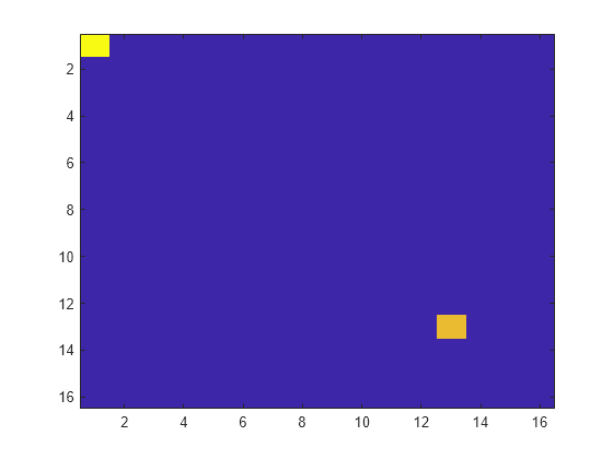
The mean component is in the top left corner of the 2-D DFT and the low negative frequency in the X and Y direction is in the lower right corner of the image as expected.
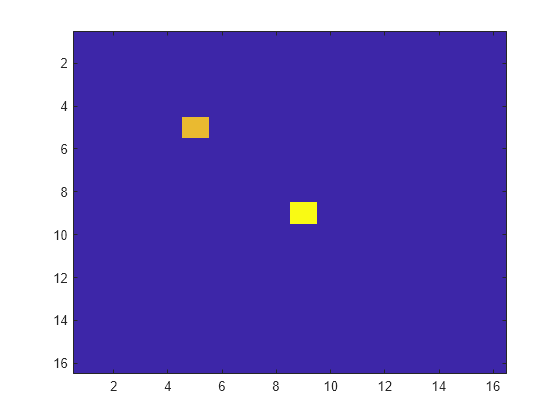
Now apply fftshift, which for matrices (images) swaps the first quadrant with the third, and the second quadrant with the fourth. This means that high negative spatial frequencies in X and Y are now in the top left corner. Spatial frequency decreases in the Y direction to zero and then increases again up to the Nyquist as you move down the image. Similarly, spatial frequencies in X decrease as you move along the image to the right until zero and then increase up to the Nyquist. The (0,0) spatial frequency component is moved to the center of the image.
imagesc(abs(fftshift(Zdft)))
The frequency ordering of the shearlet filters returned by the filterbank function follows this shifted convention for the spatial frequencies in X, but the convention is flipped for spatial frequencies in Y. Spatial frequencies in Y are large and positive in the top left corner, decrease toward zero as you move down the rows, and increase again toward large negative spatial frequencies. Accordingly, the Y spatial frequencies are flipped with respect to MATLAB's fftshift output. This has no impact on the computation of the shearlet coefficients. This needs to be taken into account only when visualizing the shearlet filters in the 2-D frequency domain.
Real-Valued Band-Limited Shearlets and Symmetry in Frequency
Obtain a real-valued shearlet system with the default image size of 128-by-128. Visualize the three horizontal cone-adapted shearlets for shearing factors of -1,0,1, respectively, at the coarsest spatial scale (finest spatial frequency resolution).
sls = shearletSystem;
[psi,scale,shear,cone] = filterbank(sls);
omegax = -1/2:1/128:1/2-1/128;
omegay = -1/2:1/128:1/2-1/128;
figure
subplot(2,2,1)
surf(omegax,flip(omegay),psi(:,:,2),'EdgeColor',"none")
view(0,90)
title('Horizontal Cone — Shear = -1')
xlabel('$\omega_x$','Interpreter',"latex",'FontSize',14)
ylabel('$\omega_y$','Interpreter',"latex","FontSize",14)
subplot(2,2,2)
surf(omegax,flip(omegay),psi(:,:,3),'EdgeColor',"none")
xlabel('$\omega_x$',"Interpreter","latex",'FontSize',14)
ylabel('$\omega_y$',"Interpreter","latex","FontSize",14)
view(0,90)
title('Horizontal Cone — Shear = 0')
subplot(2,2,3)
surf(omegax,flip(omegay),psi(:,:,4),'EdgeColor',"none")
xlabel('$\omega_x$',"Interpreter","latex","FontSize",14)
ylabel('$\omega_y$',"Interpreter","latex","FontSize",14)
view(0,90)
title('Horizontal Cone — Shear = 1')
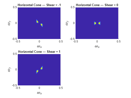
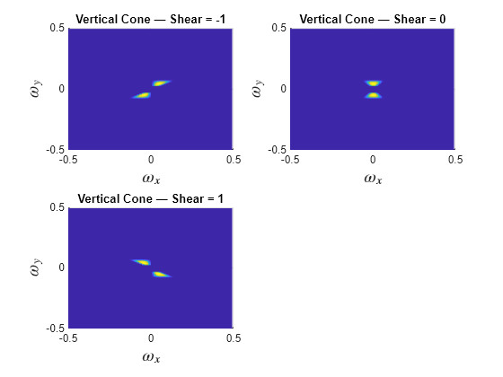
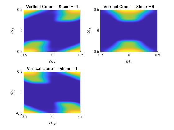
As expected and required for the shearlets to be real-valued in the spatial domain, their real-valued Fourier transforms must be symmetric with respect to the positive and negative X and Y spatial frequencies. Repeat the steps for the vertical cone-adapted shearlets at the finest spatial frequency scale.
figure
subplot(2,2,1)
surf(omegax,flip(omegay),psi(:,:,5),'EdgeColor',"none")
view(0,90)
title('Vertical Cone — Shear = -1')
xlabel('$\omega_x$','Interpreter',"latex",'FontSize',14)
ylabel('$\omega_y$','Interpreter',"latex","FontSize",14)
subplot(2,2,2)
surf(omegax,flip(omegay),psi(:,:,6),'EdgeColor',"none")
xlabel('$\omega_x$',"Interpreter","latex",'FontSize',14)
ylabel('$\omega_y$',"Interpreter","latex","FontSize",14)
view(0,90)
title('Vertical Cone — Shear = 0')
subplot(2,2,3)
surf(omegax,flip(omegay),psi(:,:,7),'EdgeColor',"none")
xlabel('$\omega_x$',"Interpreter","latex","FontSize",14)
ylabel('$\omega_y$',"Interpreter","latex","FontSize",14)
view(0,90)
title('Vertical Cone — Shear = 1')
In a square image, it is easier to ensure the required symmetry for all shearing factors and dilations than in an image where the aspect ratio differs from one. The more pronounced the difference between the height and width dimensions of an image, the harder it becomes to ensure the necessary symmetry. Ensuring perfect symmetry in the 2-D frequency plane is also harder when the shearlet overlaps the edges of the image.
In shearletSystem, the number of scales determines the support of the lowpass filter. The greater the number of the scales the more concentrated the frequency support of the lowpass filter around (0,0). For a real-valued shearlet system, the six scale-0 shearlets (3 horizontal and 3 vertical shearlets) fill in the frequency support around the lowpass filter. Accordingly, while the number of shears is constant at a given scale, the actual frequency support of the shearlets is not. To see this, construct another shearlet system with only one scale and plot the vertical-cone scale-0 shearlets.
sls1 = shearletSystem('NumScales',1);
psi1 = filterbank(sls1);
figure
subplot(2,2,1)
surf(omegax,flip(omegay),psi1(:,:,5),'EdgeColor',"none");
view(0,90)
title('Vertical Cone — Shear = -1')
xlabel('$\omega_x$','Interpreter',"latex",'FontSize',14)
ylabel('$\omega_y$','Interpreter',"latex","FontSize",14)
subplot(2,2,2)
surf(omegax,flip(omegay),psi1(:,:,6),'EdgeColor',"none");
xlabel('$\omega_x$',"Interpreter","latex",'FontSize',14)
ylabel('$\omega_y$',"Interpreter","latex","FontSize",14)
view(0,90)
title('Vertical Cone — Shear = 0')
subplot(2,2,3)
surf(omegax,flip(omegay),psi1(:,:,7),'EdgeColor',"none");
xlabel('$\omega_x$',"Interpreter","latex","FontSize",14)
ylabel('$\omega_y$',"Interpreter","latex","FontSize",14)
view(0,90)
title('Vertical Cone — Shear = 1')
In this shearlet system, the scale-0 shearlets have all their energy in the highest X and Y spatial frequencies. At these edges of the 2-D frequency plane, the symmetry required for purely real-valued shearlet coefficients can suffer numerical instabilities. The important point is that the scale at which this can happen depends on the number of scales in the shearlet system as well as the aspect ratio of the analyzed image.
Plot the frequency responses of the lowpass filter and six shearlet filters to show how the 2-D frequency plane is filled ensuring a perfect reconstruction system.
figure
for ns = 1:size(psi1,3)
    surf(omegax,flip(omegay),psi1(:,:,ns),'edgecolor','none');
    xlabel('$\omega_x$','Interpreter',"latex","FontSize",14)
    ylabel('$\omega_y$','Interpreter',"latex",'FontSize',14)
    view(0,90);
    hold on;
end
title('One-Scale Shearlet Transform Filters')
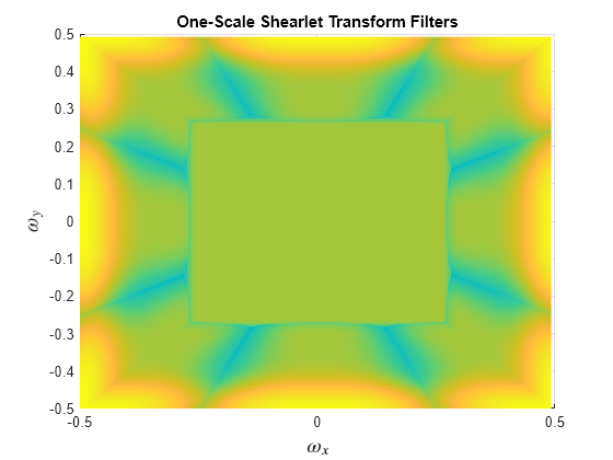
With only one scale in the shearlet system, the six shearlets must fill any region of the 2-D frequency space not covered by the lowpass filter. Accordingly, a breakdown in the symmetry required for purely real-valued shearlet coefficients may occur when there is only one scale present because those shearlets have support overlapping the edges. The next section discusses two ways to guard against the appearance of complex-valued coefficients in a real-valued shearlet transform.
Resize or Pad Rectangular Images
Whenever possible use square images. It is easier to ensure perfect symmetry in the shearlet frequency response when the aspect ratio is one. This is true even when the shearlet filters overlap the edge of the image. Read in the following image and display the image and its size.
im = imread('pout.tif');
size(im)
ans = 1×2
291 240
figure
imshow(im)
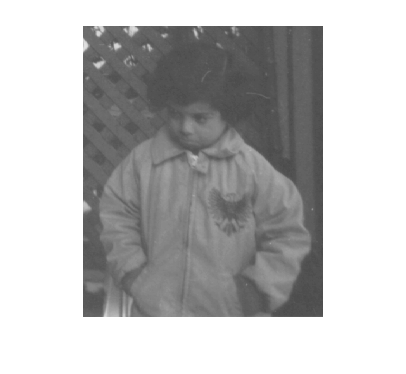
The image is 291-by-240. The default number of scales in the shearlet transform for this image size is 4. Obtain the real-valued shearlet transform for the default number of scales. Check whether any of the coefficients have a nonzero imaginary part.
sls = shearletSystem('ImageSize',size(im));
cfs = sheart2(sls,double(im));
max(imag(cfs(:)))
ans = 0
~any(imag(cfs(:)))
ans = logical
1
The shearlet coefficients are purely real-valued as expected. Repeat the steps with the maximum number of scales equal to 2.
sls = shearletSystem('ImageSize',size(im),'NumScales',2); cfs = sheart2(sls,double(im)); max(imag(cfs(:)))
ans = 9.7239e-05
~any(imag(cfs(:)))
ans = logical
0
Now the shearlet coefficients are not purely real. The perfect reconstruction property of the transform is not affected.
imrec = isheart2(sls,cfs); max(abs(imrec(:)-double(im(:))))
ans = 2.1316e-13
However, the presence of complex-valued shearlet coefficients may be undesirable.
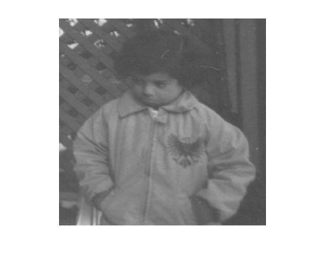
One strategy to mitigate this if you want a transform with two scales is to resize the image to 291-by-291.
imr = imresize(im,[291 291]); imshow(imr)
sls = shearletSystem('ImageSize',size(imr),'NumScales',2); cfs = sheart2(sls,double(imr)); max(imag(cfs(:)))
ans =
0
~any(imag(cfs(:)))
ans = logical
   1
By simply resizing the image to have an aspect ratio equal to one, you are able to obtain a purely real shearlet transform with the desired number of scales.
As an alternative to resizing, you can simply pad the image to the desired size. Use the wextend function to zero-pad the image columns to 291. Obtain the shearlet transform of the zero-padded image and verify that the coefficients are purely real. If you are interested only in the analysis coefficients, you can discard any padding after obtaining the shearlet transform. This is because the shearlet coefficient images have the same spatial resolution as the original image.
impad = wextend('ac','zpd',im,51,'r'); cfs = sheart2(sls,double(impad)); max(imag(cfs(:)))
ans =
0
~any(imag(cfs(:)))
ans = logical
   1
Adjust Number of Scales
There are cases where simply increasing or decreasing the number of scales by one is enough to eliminate any edge effects in the symmetry of the shearlet transform. For example, with the original image, simply incrementing the number of scales by one results in purely real-valued coefficients.
sls = shearletSystem('ImageSize',size(im),'NumScales',3); cfs = sheart2(sls,double(im)); max(imag(cfs(:)))
ans =
0
~any(imag(cfs(:)))
ans = logical
   1
References
[1] Häuser, Sören, and Gabriele Steidl. "Fast Finite Shearlet Transform: A Tutorial." arXiv preprint arXiv:1202.1773 (2014).
[2] Voigtlaender, Felix, and Anne Pein. "Analysis vs. Synthesis Sparsity for -Shearlets." arXiv preprint arXiv:1702.03559 (2017).
See Also
shearletSystem | sheart2 | isheart2