Perform 6-DoF Pose Estimation for Bin Picking Using Deep Learning

This example uses:

This example shows how to perform six degrees-of-freedom (6-DoF) pose estimation by estimating the 3-D position and orientation of machine parts in a bin using RGB-D images and a deep learning network.

6-DoF pose is the rotation and translation of an object in three-dimensional space with respect to a reference frame. 6-DoF pose estimation using images and depth sensors is key to many computer vision systems, such as intelligent bin picking, for robotics and augmented reality. In intelligent bin picking, the 6-DoF pose is the rotation and translation of an object from some canonical pose to the pose observed by a camera capturing the scene. A robotic arm paired with an RGB-D sensor, which captures both an RGB image and a depth measurement, can then use the 6-DoF pose estimation model to simultaneously detect and estimate the position and orientation of the objects with respect to the RGB-D sensor. You can use the estimated poses in downstream tasks, such as planning a path to an object or determining how to best grip an object with a particular robot gripper.

In this example, you perform 6-DoF pose estimation in three stages using a pretrained Pose Mask R-CNN network, which is a type of convolutional neural network designed for 6-DoF pose estimation [1][2]. You first train the network on an instance segmentation task to predict bounding boxes, class labels, and segmentation masks. Then, you train the network on a pose estimation task to predict 3-D rotation and translation for detected objects. To refine initial pose predictions and evaluate the results against the ground truth pose, you visualize the network predictions and apply geometry-based postprocessing. In the third stage, you train this trained model again to refine the rotation predictions for enhanced accuracy.

This example requires the Computer Vision Toolbox™ Model for Pose Mask R-CNN 6-DoF Pose Estimation. You can install the Computer Vision Toolbox Model for Pose Mask R-CNN 6-DoF Object Pose Estimation from Add-On Explorer. For more information about installing add-ons, see Get and Manage Add-Ons. The Computer Vision Toolbox Model for Pose Mask R-CNN 6-DoF Object Pose Estimation requires Deep Learning Toolbox™ and Image Processing Toolbox™.

Load Sample Data

Load a sample RGB image, and its associated depth image and camera intrinsic parameters, into the workspace.

imRGB = imread("image_00050.jpg");
load("depth_00050.mat","imDepth")
load("intrinsics_00050.mat","intrinsics")

Load the 3-D point cloud models of the object shapes, which represent machine parts, into the workspace.

load("pointCloudModels.mat","modelClassNames","modelPointClouds")

Visualize the 3-D point cloud models of the object shapes.

figure
tiledlayout(2,2,'TileSpacing','Compact')
for i = 1:length(modelPointClouds)
    nexttile
    ax = pcshow(modelPointClouds(i));
    title(modelClassNames(i), Interpreter='none')
end
sgtitle("Reference Objects", Color='w');

The ground truth annotations associated with this sample, which are bounding boxes, classes, segmentation masks and 6-DoF poses, are used to train the deep neural network. Load the annotations into the workspace.

load("groundTruth_00050.mat")

Visualize Ground Truth Annotations and Pose

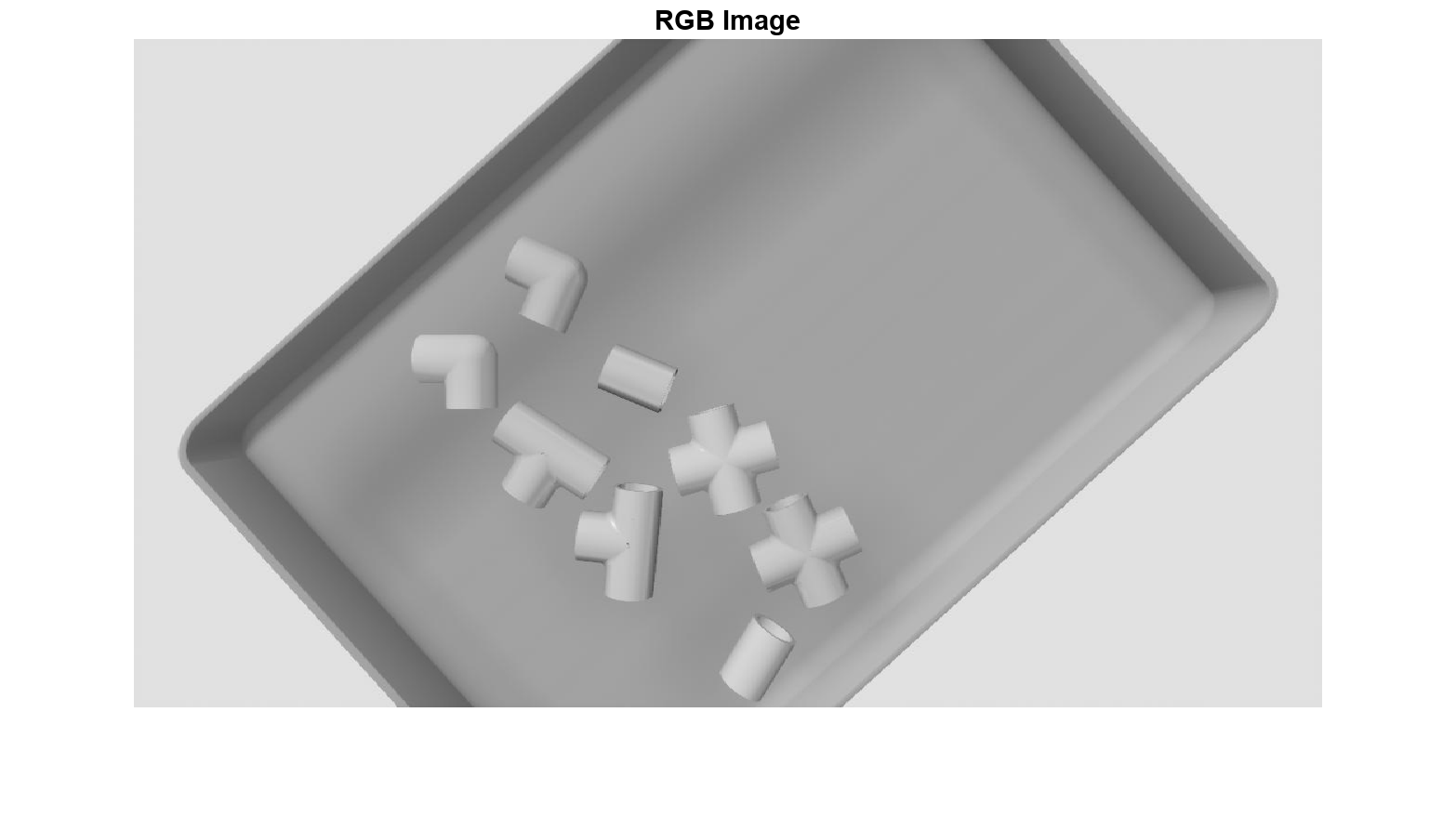
Display the sample RGB image.

figure
imshow(imRGB);
title("RGB Image")

Display the depth image. The depth image shows the distance, or depth, from the camera to each pixel in the scene.

figure
imshow(imDepth);
title("Depth Image")

Visualize Ground Truth Data

Overlay the ground truth masks on the original image using the insertObjectMask function.

imRGBAnnot = insertObjectMask(imRGB,gtMasks,Opacity=0.5);

Overlay the object bounding boxes on the original image using the insertObjectAnnotation function.

imRGBAnnot = insertObjectAnnotation(imRGBAnnot,"rectangle",gtBoxes,gtClasses);

Display the ground truth masks and bounding boxes overlaid on the original image.

figure
imshow(imRGBAnnot); 
title("Ground Truth Annotations")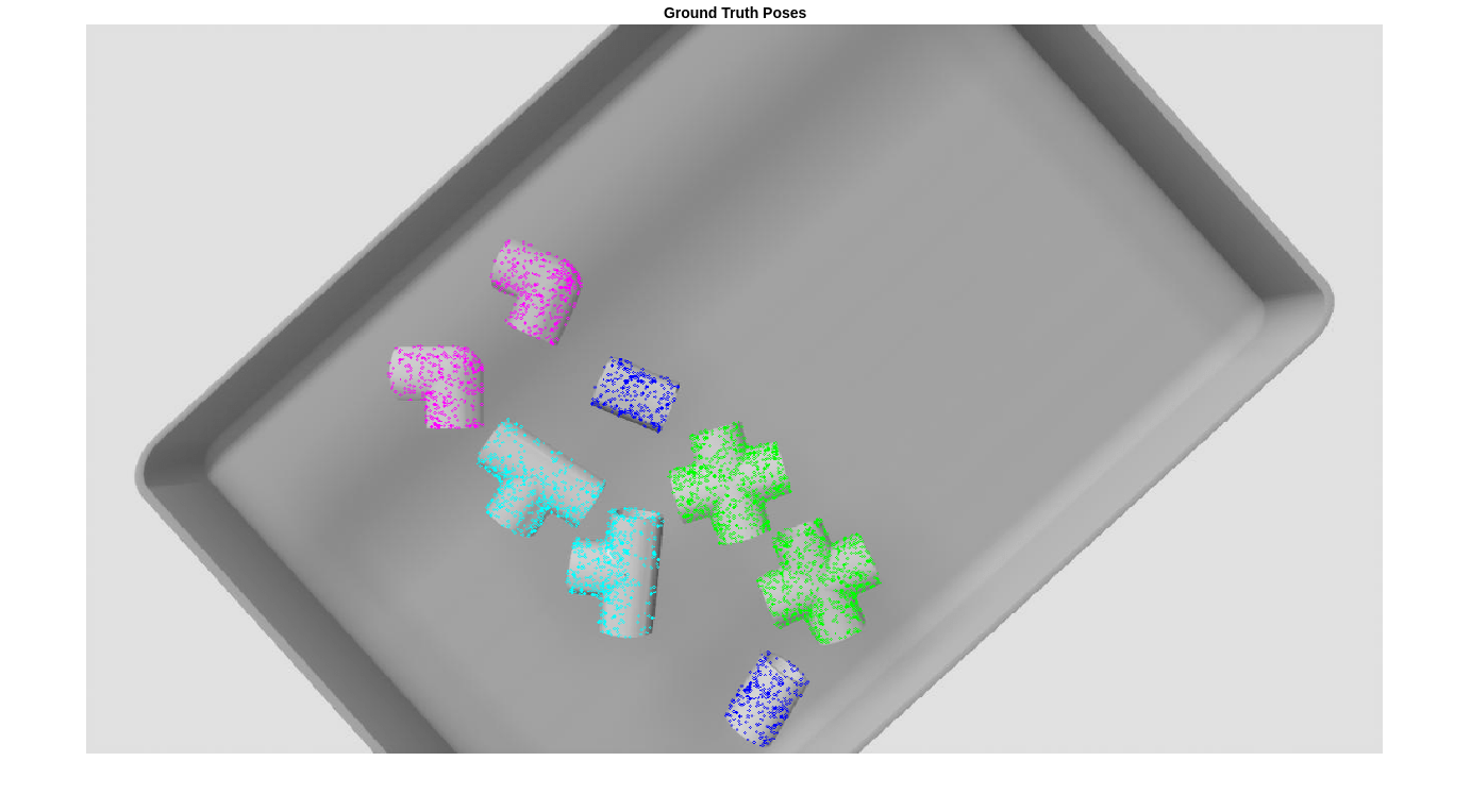

Visualize Ground Truth Pose

To visualize the 3-D rotation and translation of the objects, apply pose transformation to a point cloud of each object class, and display the point clouds on the original image. The pose-transformed point clouds, when projected onto the image, align perfectly with the orientations of the machine parts in the scene.

Define the pose colors corresponding to each object class, number of pose colors, number of objects, and create a copy of the RGB image, imGTPose, to contain the pose-transformed point clouds.

poseColors = ["blue","green","magenta","cyan"];
numPoseColors = length(poseColors);
numObj = size(gtBoxes,1);  
imGTPose = imRGB;

To visualize the ground truth object poses, display the projected point clouds overlaid on the sample image by using the helperVisualizePosePrediction supporting function..

gtPredsImg = helperVisualizePosePrediction(gtPoses, ...
    gtClasses, ...
    ones(size(gtClasses)), ...
    gtBoxes, ...
    modelClassNames, ...
    modelPointClouds, ...
    poseColors, ...
    imRGB, ...
    intrinsics);

figure
imshow(gtPredsImg);
title("Ground Truth Point Clouds")

Predict 6-DoF Pose Using Pretrained Pose Mask R-CNN Model

Create a pretrained Pose Mask R-CNN model using the posemaskrcnn object.

pretrainedNet = posemaskrcnn("resnet50-pvc-parts");

Predict the 6-DoF poses of the machine parts in the image using the predictPose object function. Specify the prediction confidence threshold Threshold as 0.5. Specify the prediction confidence threshold Threshold as 0.5.

[poses,labels,scores,boxes,masks] = predictPose(pretrainedNet, ...
                imRGB,imDepth,intrinsics,Threshold=0.5, ...
                ExecutionEnvironment="auto");

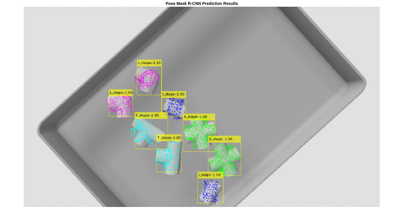
Visualize Predicted Results

Display the 6-DoF pose predictions using projected point clouds, as used to visualize the ground truth poses in the Visualize Ground Truth Pose section of this example. To visualize the predicted object poses, display the projected point clouds overlaid on the sample image by using the helperVisualizePosePrediction supporting function.

pretrainedPredsImg = helperVisualizePosePrediction(poses, ...
    labels, ...
    scores, ...
    boxes, ...
    modelClassNames, ...
    modelPointClouds, ...
    poseColors, ...
    imRGB, ...
    intrinsics);

figure;
imshow(pretrainedPredsImg);
title("Pose Mask R-CNN Prediction Results")

By visualizing the Pose Mask R-CNN network predictions in this way, you can see that the network correctly predicts the 2-D bounding boxes and classes, as well as the 3-D translations of the parts in the bin. Because 3-D rotation is a more challenging task, the predictions are a bit noisy. To refine the results, combine the deep learning results with traditional point cloud processing techniques in the Refine Estimated Pose section.

Refine Estimated Pose

Obtain Partial Point Clouds from Depth Image

To improve the accuracy of the predictions from the Pose Mask R-CNN network, combine the predicted poses with traditional geometric processing of the point cloud data. In this section, use the depth image and the camera intrinsic parameters to obtain a point cloud representation of the scene.

Use postprocessing to remove points that are too far away to realistically be part of the bin-picking scene, such as points on a far wall or floor. Specify this reasonable maximum distance from the camera, or maximum depth, as 0.5.

maxDepth = 0.5;

To help remove the surface of the bin on which the PVC parts are resting from the point cloud data, fit a 3-D plane to the bin surface in the scene point cloud. Specify the maximum bin distance and the bin orientation for the plane-fitting procedure. The maximum bin distance is an estimate of the largest distance from the bin to the camera. For simplicity, assume the bin is in a horizontal orientation.

maxBinDistance = 0.0015;
binOrientation = [0 0 -1];

Postprocess the raw scene point cloud from the depth image and return point clouds for each detected object by using the helperPostProcessScene supporting function.

[scenePointCloud,roiScenePtCloud] = helperPostProcessScene(imDepth,intrinsics,boxes,maxDepth, ...
    maxBinDistance,binOrientation);

Plot the scene point cloud.

figure;
pcshow(scenePointCloud,VerticalAxisDir="Down")
title("Scene Point Cloud from Depth Image")

Plot one of the object point clouds extracted from the depth image.

figure;
pcshow(roiScenePtCloud{end}, VerticalAxisDir="Down")

title("Object Point Cloud from Depth Image")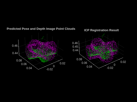

Register Point Clouds to Refine Pose Estimation

To refine pose estimation results, perform point cloud registration based on the iterative closest point (ICP) algorithm using the pcregistericp function. During registration, you align the object poses predicted by the Pose Mask R-CNN model with partial point clouds of objects from the depth image. To reduce the number of point cloud points used and improve computation time, use the pcdownsample function and set the downsample factor to 0.25.

downsampleFactor = 0.25;
numPreds = size(boxes,1); 
registeredPoses = cell(numPreds,1);
for detIndex = 1:numPreds
    detClass = string(labels(detIndex));

    % Define predicted rotation and translation.
    detTform = poses(detIndex);
    detScore = scores(detIndex);
    
    % Retrieve the 3-D object point cloud of the predicted object class.
    ptCloud = modelPointClouds(modelClassNames == detClass);
    
    % Transform the 3-D object point cloud using the predicted pose.
    ptCloudDet = pctransform(ptCloud, detTform);
    
    % Downsample the object point cloud transformed by the predicted pose.
    ptCloudDet = pcdownsample(ptCloudDet,"random",downsampleFactor);

    % Downsample point cloud obtained from the postprocessed scene depth image.
    ptCloudDepth =  pcdownsample(roiScenePtCloud{detIndex},"random",downsampleFactor);
    
    % Run the ICP point cloud registration algorithm with default
    % parameters.
    [tform,movingReg] = pcregistericp(ptCloudDet,ptCloudDepth);
    registeredPoses{detIndex} = tform;
end

For simplicity, visualize the registration for a single detected object. In the left subplot, plot the point clouds obtained from the Pose Mask R-CNN predictions in magenta and those from postprocessing of the scene depth image in green in the left subplot. In the right subplot, plot the registered point cloud in magenta and the depth image point cloud in green.

figure
subplot(1,2,1)
pcshowpair(ptCloudDet,ptCloudDepth)
title("Predicted Pose and Depth Image Point Clouds")

subplot(1,2,2)
pcshowpair(movingReg,ptCloudDepth)
title("ICP Registration Result")

Combine Pose Mask R-CNN Predicted Pose with Point Cloud Registration

Visualize the poses predicted by the Pose Mask R-CNN network after the postprocessing and refinement steps, which are now significantly improved. Store the 6-DoF pose consisting of a rotation and a translation in three dimensions as a rigidtform3d object.

refinedPoses = cell(1,numPreds);

for detIndex = 1:numPreds 

    detClass = string(labels(detIndex));

    % Define predicted rotation and translation.
    detTform = poses(detIndex);
    detScore = scores(detIndex);

    % Rotation and translation from registration of depth point clouds.
    icpTform = registeredPoses{detIndex};

    % Combine the two transforms to return the final pose.
    combinedTform = rigidtform3d(icpTform.A*detTform.A);
    refinedPoses{detIndex} = combinedTform;

end
refinedPoses = cat(1,refinedPoses{:});

imPoseRefined = helperVisualizePosePrediction(refinedPoses, ...
    labels, ...
    scores, ...
    boxes, ...
    modelClassNames, ...
    modelPointClouds, ...
    poseColors, ...
    imRGB, ...
    intrinsics);

figure
imshow(imPoseRefined);
title("Pose Mask R-CNN + ICP")

The projected points are now more aligned to the machine parts present in the image, and the rotation results are more accurate.

Evaluate 6-DoF Pose Prediction

To quantify or evaluate the quality of predicted 6-DoF object poses, use the Chamfer distance [3] to measure the distance between the closest points of a point cloud transformed by the predicted pose and the same point cloud transformed by the ground truth pose. A small Chamfer distance indicates that the predicted and ground truth poses match closely. To demonstrate a closer pose alignment at a shorter Chamfer distance, display all the object point clouds as ground truth (green) and predicted (magenta) poses.

First, calculate the Chamfer distance between the object point clouds in the ground truth and predicted poses by using the helperEvaluatePosePrediction supporting function.

[distPtCloud,predIndices,gtIndices] = helperEvaluatePosePrediction( ...
    modelPointClouds,modelClassNames,boxes,labels,refinedPoses,gtBoxes,gtClasses,gtPoses);

helperVisualizeChamferDistance(...
    labels, predIndices, gtIndices, modelPointClouds, ...
    modelClassNames, gtClasses, refinedPoses, gtPoses, distPtCloud);

avgChamferDistance = mean(distPtCloud(:));
sgtitle(["Pose Mask R-CNN Chamfer Distances" "Mean " + num2str(avgChamferDistance)], Color='w');

Prepare Data for Training

Perform transfer learning on a custom bin-picking data set using the Pose Mask R-CNN deep learning network. The data set contains 100 RGB images and depth images of 3-D pipe connectors, generated using Simulink®. The data consists of images of these machine parts lying at random orientations inside a bin, viewed from different angles and under different lighting conditions, and contains four object classes that correspond to objects having I, X, L, or T shapes. The data set additionally contains bounding boxes, object classes, binary masks, and 6-DoF pose information for every object in each image, as well as point cloud data for each of the four object classes.

Download Data Set

Download the data set using the supporting function helperDownloadPVCPartsDataset. This step requires an internet connection.

datasetUnzipFolder = helperDownloadPVCPartsDataset;

Load and Partition Data

Prior to partitioning the data, set the global random state to ensure a higher reproducibility of results.

rng("default");

Specify the location of the data set and ground truth data.

datasetDir = fullfile(datasetUnzipFolder,"pvcparts100");
gtLocation = fullfile(datasetDir,"GT");

Create a fileDatastore object by using the helperSimAnnotMATReader supporting function that reads from the bin-picking data set.

dsRandom = fileDatastore(gtLocation, ...
    ReadFcn=@(x)helperSimAnnotMATReader(x,datasetDir));

Split the data set randomly into training and validation sets. Because the total number of images is relatively small, allocate a relatively large percentage (70%) of the data for training, and 30% for validation.

randIndices = randperm(length(dsRandom.Files));
numTrainRandom = round(0.7*length(dsRandom.Files)); 
dsTrain = subset(dsRandom,randIndices(1:numTrainRandom));
dsVal = subset(dsRandom,randIndices(numTrainRandom+1:end));

Use the data loader to query the RGB image, depth image, object masks, object classes, bounding boxes, poses, and camera intrinsic parameters of first validation sample.

data = preview(dsVal);
imRGB = data{1};
imDepth = data{2};
gtMasks = data{5};
gtClasses = data{4};
gtBoxes = data{3};
gtPoses = data{6};
intrinsics = data{7};

Ensure that the queried object classes maintain the correct order.

trainClassNames = categories(gtClasses)

trainClassNames = 4×1 cell
    {'I_shape'}
    {'X_shape'}
    {'L_shape'}
    {'T_shape'}

Train Pose Mask R-CNN Network

Train the Pose Mask R-CNN model in three stages:

Train the pretrained Pose Mask R-CNN network on the instance segmentation task, which consists of predicting bounding boxes, class labels and segmentation masks. This first training step initializes the deep neural network weights.
Train the trained Pose Mask R-CNN network from the previous step on the pose estimation task, which consists of predicting 3-D rotation and translation for each object detected.
Train the trained Pose Mask R-CNN Network from the previous step on the pose estimation task to refine rotation predictions.

Train on one or more GPUs, if they are available. Training on GPU is strongly recommended to obtain reasonable speeds. Using a GPU requires a Parallel Computing Toolbox™ license and a CUDA®-enabled NVIDIA® GPU. For more information, see GPU Computing Requirements (Parallel Computing Toolbox).

The three stages of training take approximately 15, 15, and 70 minutes, respectively, on an NVIDIA GeForce RTX 2080 Ti GPU.

Estimate Anchor Boxes

To train the Pose Mask R-CNN network, set the doTrain variable below to true. To train the network on your custom data set, estimate the anchor box locations which are specific to the data. Estimate the bounding boxes from a subset of 100 training images. Estimate the anchor boxes using the estimateAnchorBoxes function.

doTrain = false;

if doTrain
    numAnchors = 8;
    numImgSample = 100;
    numImgSample = min(numImgSample, length(dsTrain.Files));
    sampledBboxes = {};
    dsTmp = copy(dsTrain);
    for ii=1:numImgSample
        tmpData = read(dsTmp);
        randSelect = randi(size(tmpData{3},1));
        sampledBboxes{end+1} = tmpData{3}(randSelect,:);
    end
    blds = boxLabelDatastore(table(sampledBboxes'));
    [anchorBoxes,meanAnchorIoU] = estimateAnchorBoxes(blds,numAnchors);
end

Define Pose Mask R-CNN Network Architecture

Create the Pose Mask R-CNN pose estimation network using the posemaskrcnn object. Specify the pretrained network created using ResNet-50 as the base network. Specify the class names and the estimated anchor boxes.

if doTrain
    untrainedNetwork = posemaskrcnn("resnet50-pvc-parts",trainClassNames,anchorBoxes);
end

Training Stage 1: Perform Instance Segmentation

Specify Training Options

Specify network training options for the instance segmentation training stage using the trainingOptions (Deep Learning Toolbox) function. Train the object detector using the SGDM solver for a maximum of 5 epochs. Specify the ValidationData name-value argument as the validation data dsVal. Specify the location to save intermediate network checkpoints.

if doTrain
    outFolder = fullfile(tempdir,"output","train_posemaskrcnn_stage1");
    mkdir(outFolder);
    ckptFolder = fullfile(outFolder, "checkpoints");
    mkdir(ckptFolder);
    disp(outFolder);
    
    optionsStage1 = trainingOptions("sgdm", ...
        InitialLearnRate=0.0001, ...  
        LearnRateSchedule="piecewise", ...
        LearnRateDropPeriod=1, ...
        LearnRateDropFactor=0.5, ...
        MaxEpochs=5, ...
        Plot="none", ...
        Momentum=0.9, ...
        MiniBatchSize=1, ... 
        ResetInputNormalization=false, ...
        ExecutionEnvironment="auto", ...
        VerboseFrequency=5, ...
        ValidationData=dsVal, ...
        ValidationFrequency=20, ...
        Plots="training-progress", ...
        CheckpointPath=ckptFolder,...
        CheckpointFrequency=2,...
        CheckpointFrequencyUnit="epoch");
end

/tmp/output/train_posemaskrcnn_stage1

Train Pose Mask R-CNN

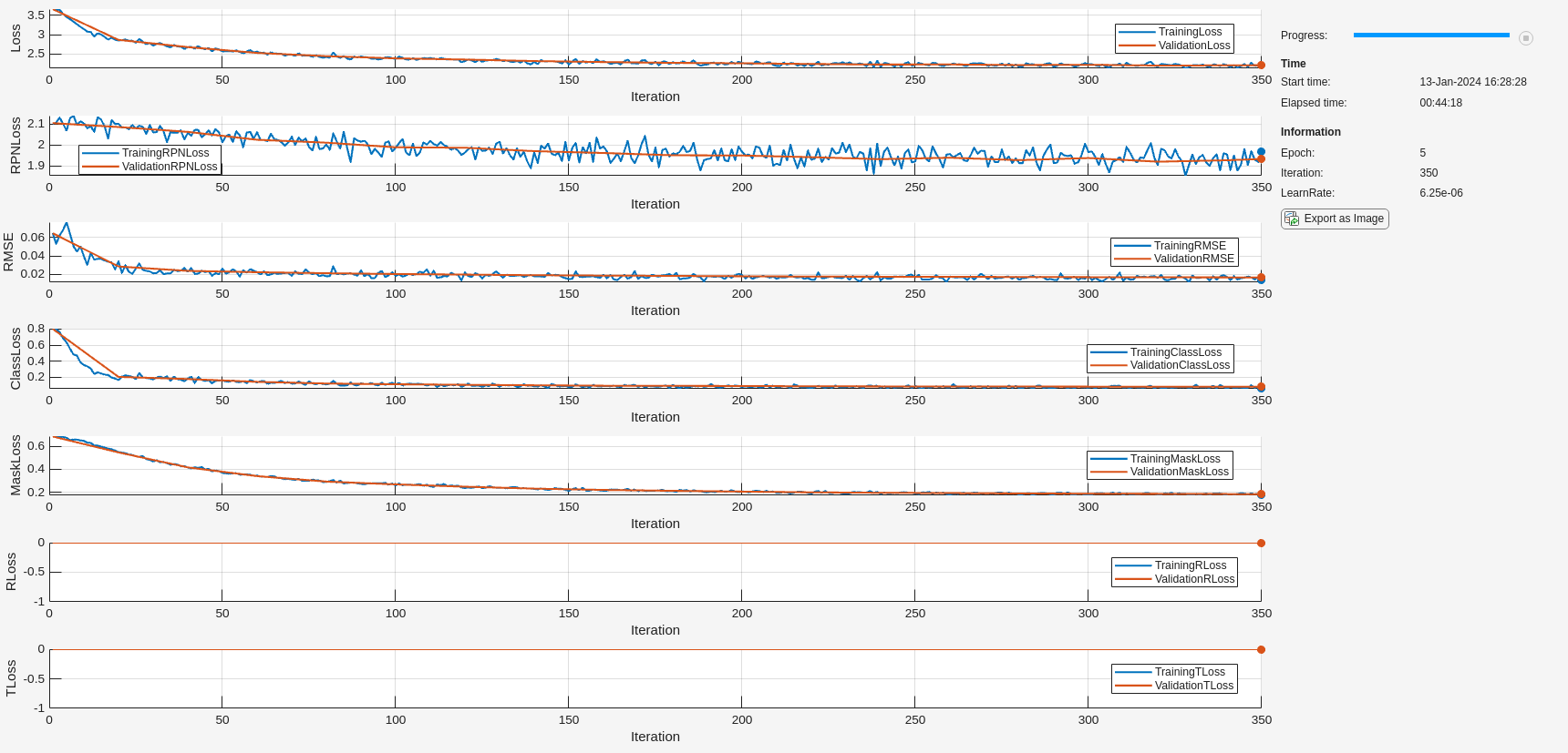
Train the Pose Mask R-CNN network to predict bounding boxes, object classes, and instance segmentation masks using the trainPoseMaskRCNN function. This training step does not use pose or mask head losses. Save the trained network to a local folder and plot the progress of the training loss over multiple iterations.

if doTrain
    [net, info] = trainPoseMaskRCNN(...
        dsTrain,untrainedNetwork,"mask",optionsStage1); 
    
    modelDateTime = string(datetime("now", Format='yyyy-MM-dd-HH-mm-ss'));
    save(fullfile(outFolder,"stage1trainedPoseMaskRCNN-"+modelDateTime+".mat"),"net");
    disp(fullfile(outFolder,"stage1trainedPoseMaskRCNN-"+modelDateTime+".mat"))
end

Training Stage 2: Predict Pose

Specify Training Options

Specify network training options for the pose prediction training stage using the trainingOptions (Deep Learning Toolbox) function. Train the object detector using the SGDM solver for a maximum of 5 epochs. Specify the ValidationData name-value argument as the validation data dsVal. Specify the location to save intermediate network checkpoints. Apply regression losses for 3D translation and rotation to train the network in this stage.

if doTrain
    outFolder = fullfile(tempdir,"output","train_posemaskrcnn_stage2");
    mkdir(outFolder);
    ckptFolder = fullfile(outFolder,"checkpoints");
    mkdir(ckptFolder);
    disp(outFolder);

    optionsStage2 = trainingOptions("sgdm", ...
        InitialLearnRate=0.0001, ...  
        LearnRateSchedule="piecewise", ...
        LearnRateDropPeriod=1, ...
        LearnRateDropFactor=0.5, ...
        MaxEpochs=5, ...
        Plot="none", ...
        Momentum=0.9, ...
        MiniBatchSize=1, ... 
        ResetInputNormalization=false, ...
        ExecutionEnvironment="auto", ...
        VerboseFrequency=5, ...
        ValidationData=dsVal, ...
        ValidationFrequency=20, ...
        Plots="training-progress", ...
        CheckpointPath=ckptFolder,...
        CheckpointFrequency=5,...
        CheckpointFrequencyUnit="epoch");
end

/tmp/output/train_posemaskrcnn_stage2

Train Pose Mask R-CNN

To predict 6-DoF pose for every detected object, train the Pose Mask R-CNN network trained for instance segmentation, net, with both pose and mask losses using the trainPoseMaskRCNN function. Save the trained network to a local folder and plot the progress of the training loss for rotation and translation over multiple iterations.

if doTrain
    trainedNet = trainPoseMaskRCNN(...
        dsTrain,net,"mask-and-pose",optionsStage2);  
    
    modelDateTime = string(datetime("now",Format="yyyy-MM-dd-HH-mm-ss"));
    save(fullfile(outFolder,"stage2trainedPoseMaskRCNN-"+modelDateTime+".mat"),"trainedNet");
    disp(fullfile(outFolder,"stage2trainedPoseMaskRCNN-"+modelDateTime+".mat"))
    
end

Estimate Pose

Predict the 6-DoF poses of the machine parts in the image using the predictPose object function. Specify the prediction confidence threshold Threshold as 0.5.

if doTrain
    [poses,labels,scores,boxes,masks] = predictPose(trainedNet, ...
                data{1},data{2},data{end},Threshold=0.5, ...
                ExecutionEnvironment="auto");

Visualize pose predictions.

    image = data{1};
    intrinsics = data{end};
    trainedPredsImg = helperVisualizePosePrediction(poses, ...
        labels, ...
        scores, ...
        boxes, ...
        modelClassNames, ...
        modelPointClouds, ...
        poseColors, ...
        image, ...
        intrinsics);
    
    figure;
    imshow(trainedPredsImg);
    title("Pose Mask R-CNN Prediction Results After Stage 2")
end

To evaluate the 6-DoF pose prediction, calculate the Chamfer distance between the object point clouds in the ground truth and predicted poses by using the helperEvaluatePosePrediction supporting function.

if doTrain
    [distPtCloud,predIndices,gtIndices] = helperEvaluatePosePrediction( ...
        modelPointClouds,modelClassNames,boxes,labels,poses,gtBoxes,gtClasses,gtPoses);
end

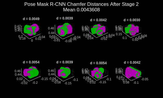
Next, visualize the point cloud pairs in ground truth and predicted poses, and display the Chamfer distance value corresponding to each object pose using the helperVisualizeChamferDistance supporting function. While the translation predictions look correct, the predicted rotations do not align well compared to the ground truth poses.

if doTrain
    helperVisualizeChamferDistance(...
        labels, predIndices, gtIndices, modelPointClouds, ...
        modelClassNames, gtClasses, poses, gtPoses, distPtCloud);
    
    avgChamferDistance = mean(distPtCloud(:));
    sgtitle(["Pose Mask R-CNN Chamfer Distances After Stage 2" "Mean " + num2str(avgChamferDistance)], Color='w');
end

Training Stage 3: Refine Pose

After the model has been trained for instance segmentation and pose estimation, train the model in a third stage to refine rotation predictions and account for object symmetry.

Specify Training Options

Specify network training options for the pose refinement training stage using the trainingOptions (Deep Learning Toolbox) function. Train the object detector using the SGDM solver for a maximum of 10 epochs. Specify the ValidationData name-value argument as the validation data dsVal. Specify the location to save intermediate network checkpoints.

if doTrain
    outFolder = fullfile(tempdir,"output","train_posemaskrcnn_stage3");
    mkdir(outFolder);
    ckptFolder = fullfile(outFolder,"checkpoints");
    mkdir(ckptFolder);
    disp(outFolder);

    optionsStage3 = trainingOptions("sgdm", ...
        InitialLearnRate=0.0001, ...  
        LearnRateSchedule="piecewise", ...
        LearnRateDropPeriod=1, ...
        LearnRateDropFactor=0.5, ...
        MaxEpochs=10, ...
        Plot="none", ...
        Momentum=0.9, ...
        MiniBatchSize=1, ... 
        ResetInputNormalization=false, ...
        ExecutionEnvironment="auto", ...
        VerboseFrequency=5, ...
        ValidationData=dsVal, ...
        ValidationFrequency=20, ...
        Plots="training-progress", ...
        CheckpointPath=ckptFolder, ...
        CheckpointFrequency=2, ...
        CheckpointFrequencyUnit="epoch");
end

/tmp/output/train_posemaskrcnn_stage3

Train Pose Mask R-CNN

Train the Pose Mask R-CNN network trained for pose estimation, trainedNet, to refine rotation predictions using the trainPoseMaskRCNN function. Specify a much larger value for RotationLossWeight than the default value, 1, and specify the ReferencePointClouds name-value argument as the 3-D point cloud models of the object shapes. Save the trained network to a local folder and plot the progress of the training loss for rotation and translation over multiple iterations.

if doTrain
    [refinedNet,info] = trainPoseMaskRCNN(...
        dsTrain, trainedNet,"pose-refinement",optionsStage3, ...
        FreezeSubNetwork=["rpn", "backbone"], ...
        RotationLossWeight=1e6, ...
        ReferencePointClouds = modelPointClouds);
    
    modelDateTime = string(datetime("now",Format="yyyy-MM-dd-HH-mm-ss"));
    save(fullfile(outFolder,"stage3trainedPoseMaskRCNN-"+modelDateTime+".mat"),"net");
    disp(fullfile(outFolder,"stage3trainedPoseMaskRCNN-"+modelDateTime+".mat"))
end

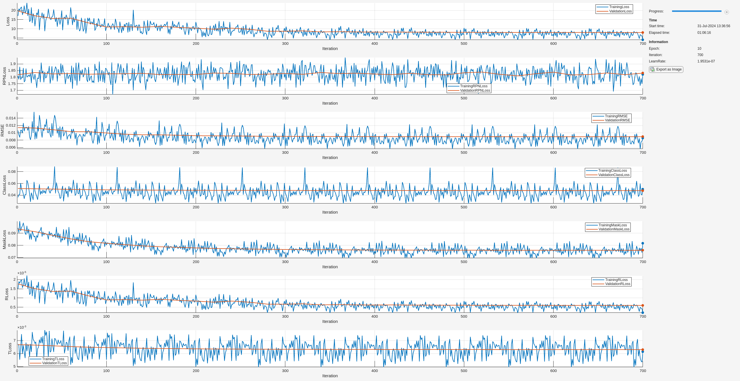
     10         700        01:05:33      1.9531e-07       3.9928           1.8211          0.0085797          0.050034             0.081616          1.97e-06         0.0061428          7.9872             1.8307            0.0089327            0.047982               0.075946           5.9604e-06          0.0063155

Estimate Pose

Predict the 6-DoF poses of the machine parts in the image using the predictPose object function. Specify the prediction confidence threshold Threshold as 0.5.

if doTrain
    [poses,labels,scores,boxes,masks] = predictPose(refinedNet, ...
                data{1},data{2},data{end},Threshold=0.5, ...
                ExecutionEnvironment="auto");

Visualize pose predictions.

    image = data{1};
    intrinsics = data{end};
    refinedPredsImg = helperVisualizePosePrediction(poses, ...
        labels, ...
        scores, ...
        boxes, ...
        modelClassNames, ...
        modelPointClouds, ...
        poseColors, ...
        image, ...
        intrinsics);
    
    figure;
    imshow(refinedPredsImg);
    title("Pose Mask R-CNN Prediction Results After Stage 3")
end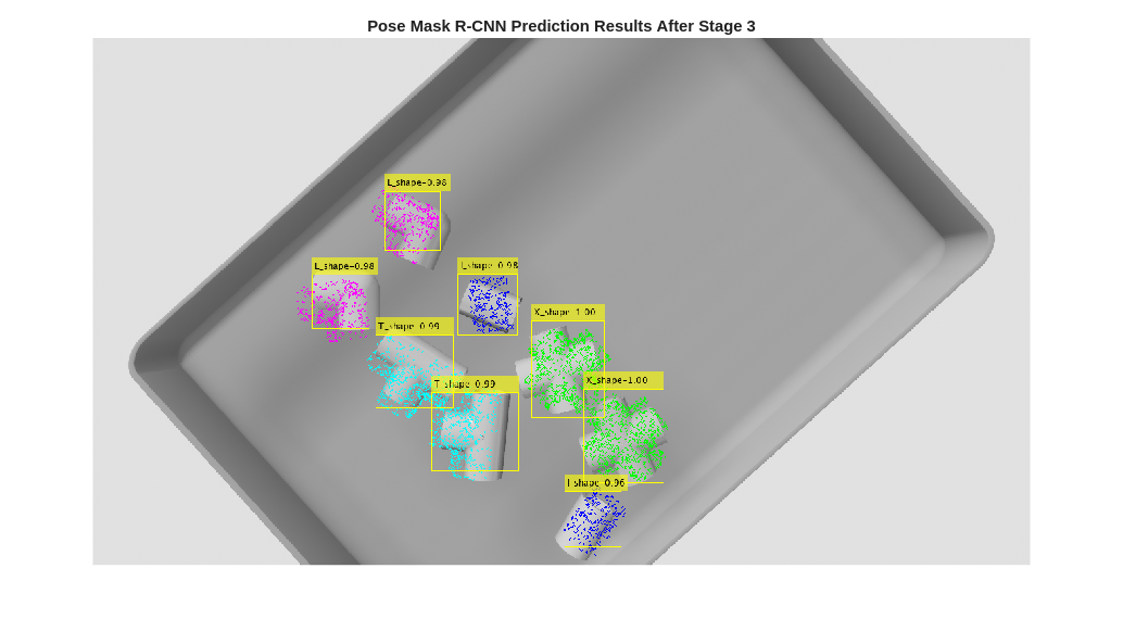

To evaluate the refined 6-DoF pose prediction, calculate the Chamfer distance between the object point clouds in the ground truth and refined predicted poses by using the helperEvaluatePosePrediction supporting function.

if doTrain
    [distPtCloud,predIndices,gtIndices] = helperEvaluatePosePrediction( ...
        modelPointClouds,modelClassNames,boxes,labels,poses,gtBoxes,gtClasses,gtPoses);
end

Next, visualize the point cloud pairs in ground truth and predicted poses, and display the Chamfer distance value corresponding to each object pose using the helperVisualizeChamferDistance supporting function. The model performance improved significantly in the this stage compared to the first two stages of training. To further improve the model's rotation predictions, you can increase the number of training epochs.

if doTrain
    helperVisualizeChamferDistance(...
        labels,predIndices,gtIndices,modelPointClouds, ...
        modelClassNames,gtClasses,poses,gtPoses,distPtCloud);
    
    avgChamferDistance = mean(distPtCloud(:));
    sgtitle(["Pose Mask R-CNN Chamfer Distances After Stage 3" "Mean " + num2str(avgChamferDistance)],Color="w");
end

Supporting functions

`helperSimAnnotMATReader`

function out = helperSimAnnotMATReader(filename,datasetRoot)
% Read annotations for simulated bin picking dataset
% Expected folder structure under `datasetRoot`:
%       depth/      (depth images folder)
%       GT/         (ground truth MAT files)
%       image/      (color images)

    data = load(filename);
    groundTruthMaT = data.groundTruthMaT;
    clear data;
    
    % Read RGB image.
    tmpPath = strsplit(groundTruthMaT.RGBImagePath, '\');
    basePath = {tmpPath{4:end}};
    imRGBPath = fullfile(datasetRoot, basePath{:});
    im = imread(imRGBPath);
    im = rgb2gray(im);
    if(size(im,3)==1)
        im = repmat(im, [1 1 3]);
    end
    
    % Read depth image.
    aa = strsplit(groundTruthMaT.DepthImagePath, '\');
    bb = {aa{4:end}};
    imDepthPath = fullfile(datasetRoot,bb{:}); % handle windows paths
    imD = load(imDepthPath); imD = imD.depth;
    
    % For "undefined" value in instance labels, assign to the first class.
    undefinedSelect = isundefined(groundTruthMaT.instLabels);
    classNames = categories(groundTruthMaT.instLabels);
    groundTruthMaT.instLabels(undefinedSelect) = classNames{1};
    if isrow(groundTruthMaT.instLabels)
        groundTruthMaT.instLabels = groundTruthMaT.instLabels';
    end
    
    % Wrap the camera parameter matrix into the cameraIntrinsics object.
    K = groundTruthMaT.IntrinsicsMatrix;
    intrinsics = cameraIntrinsics([K(1,1) K(2,2)], [K(1,3)  K(2,3)], [size(im,1) size(im, 2)]);
    
    % Process rotation matrix annotations.
    rotationCell = num2cell(groundTruthMaT.rotationMatrix,[1 2]);
    rotationCell = squeeze(rotationCell);
    
    % Process translation annotations.
    translation = squeeze(groundTruthMaT.translation)';
    translationCell = num2cell(translation, 2);
    
    % Process poses into rigidtform3d vector - transpose R to obtain the
    % correct pose.
    poseCell = cellfun( @(R,t)(rigidtform3d(R',t)), rotationCell, translationCell, ...
        UniformOutput=false);
    pose = vertcat(poseCell{:});
    
    % Remove heavily occluded objects.
    if length(groundTruthMaT.occPercentage) == length(groundTruthMaT.instLabels)
        visibility = groundTruthMaT.occPercentage;
        visibleInstSelector = visibility > 0.5;
    else
        visibleInstSelector = true([length(groundTruthMaT.instLabels),1]);
    end
    
    out{1} = im;
    out{2} = imD;                                                    % HxWx1 double array depth-map
    out{3} = groundTruthMaT.instBBoxes(visibleInstSelector,:);       % Nx4 double bounding boxes
    out{4} = groundTruthMaT.instLabels(visibleInstSelector);         % Nx1 categorical object labels
    out{5} = logical(groundTruthMaT.instMasks(:,:,visibleInstSelector));      % HxWxN logical mask arrays
    out{6} = pose(visibleInstSelector);                              % Nx1 rigidtform3d vector of object poses
    out{7} = intrinsics;                                             % cameraIntrinsics object

end

`helperPostProcessScene`

function [scenePtCloud,roiScenePtCloud] = helperPostProcessScene(imDepth,intrinsics,boxes,maxDepth,maxBinDistance,binOrientation)

    % Convert the depth image into an organized point cloud using camera
    % intrinsics.
    scenePtCloud = pcfromdepth(imDepth,1.0,intrinsics);
    
    % Remove outliers, or points that are too far away to be in the bin.
    selectionROI = [...
            scenePtCloud.XLimits(1) scenePtCloud.XLimits(2) ...
            scenePtCloud.YLimits(1) scenePtCloud.YLimits(2) ...
            scenePtCloud.ZLimits(1) maxDepth];
    selectedIndices = findPointsInROI(scenePtCloud, selectionROI);
    cleanScenePtCloud = select(scenePtCloud,selectedIndices);
    
    % Fit a plane to the bin surface.
    [~,~,outlierIndices] = pcfitplane(...
        cleanScenePtCloud,maxBinDistance,binOrientation);
    
    % Re-map indices back to the original scene point cloud. Use this
    % when cropping out object detections from the scene point cloud.
    origPtCloudSelection = selectedIndices(outlierIndices);
    
    % Crop predicted ROIs from the scene point cloud.
    numPreds = size(boxes,1);
    roiScenePtCloud = cell(1,numPreds);
    for detIndex=1:numPreds
        box2D = boxes(detIndex,:);
        
        % Get linear indices into the organized point cloud corresponding to the 
        % predicted 2-D bounding box of an object.
        boxIndices = (box2D(2):box2D(2)+box2D(4))' + (size(scenePtCloud.Location,1)*(box2D(1)-1:box2D(1)+box2D(3)-1));
        boxIndices = uint32(boxIndices(:));
        
        % Remove points that are outliers from earlier pre-processing steps
        % (either belonging to the bin surface or too far away).
        keptIndices = intersect(origPtCloudSelection,boxIndices);
        roiScenePtCloud{detIndex} = select(scenePtCloud,keptIndices);
    end

end

helperVisualizeChamferDistance

function fig = helperVisualizeChamferDistance(...
    labels, predIndices, gtIndices, modelPointClouds, ...
    modelClassNames, gtClasses, poses, gtPoses, distances)
    fig = figure;

    for idx = 1:numel(predIndices)
        detIndex = predIndices(idx);

        if detIndex == 0
            % The ground truth bounding box does not match any predicted
            % bounding boxes (false negative)
            ptCloudTformDet = pointCloud(single.empty(0, 3));
        else
            detClass = string(labels(detIndex));
            gtIndex = gtIndices(idx);
    
            % Obtain the point cloud of the predicted object.
            ptCloudDet = modelPointClouds(modelClassNames == detClass);
    
            % Predicted 6-DoF pose with ICP refinement.
            detTform = poses(detIndex);
    
            % Apply the predicted pose transformation to the predicted object point
            % cloud.
            ptCloudTformDet = pctransform(ptCloudDet, detTform);
        end

        if gtIndex == 0
            % The predicted bounding box does not match any
            % ground truth bounding box (false positive).
            ptCloudTformGT = pointCloud(single.empty(0,3));
        else
            % Obtain the point cloud of the ground truth object.
            ptCloudGT = modelPointClouds(modelClassNames == string(gtClasses(gtIndex)));

            % Apply the ground truth pose transformation.
            ptCloudTformGT = pctransform(ptCloudGT,gtPoses(gtIndex));
        end

        subplot(2,4,gtIndex);
        pcshowpair(ptCloudTformDet,ptCloudTformGT);
        title(sprintf("d = %.4f",distances(idx)))
    end
end

helperVisualizePosePrediction

function image = helperVisualizePosePrediction(...
    poses, labels, scores, boxes, modelClassNames, modelPointClouds, poseColors, imageOrig, intrinsics)
    image = imageOrig;
    numPreds = size(boxes,1);  
    detPosedPtClouds = cell(1,numPreds);
    for detIndex = 1:numPreds
        
        detClass = string(labels(detIndex));
        detTform = poses(detIndex);
        
        % Retrieve the 3-D object point cloud of the predicted object class.
        ptCloud = modelPointClouds(modelClassNames == detClass);
        
        % Transform the 3-D object point cloud using the predicted pose.
        ptCloudDet = pctransform(ptCloud, detTform);
        detPosedPtClouds{detIndex} = ptCloudDet;
    
        % Subsample the point cloud for cleaner visualization.
        ptCloudDet = pcdownsample(ptCloudDet,"random",0.05);
    
        % Project the transformed point cloud onto the image using the camera
        % intrinsic parameters and identity transform for camera pose and position.
        projectedPoints = world2img(ptCloudDet.Location,rigidtform3d,intrinsics);
        
        % Overlay the 2-D projected points over the image.helperVisualizeChamferDistance
        image = insertMarker(image,[projectedPoints(:,1), projectedPoints(:,2)],...
            "circle",Size=1,Color=poseColors(modelClassNames==detClass));
    end

    % Insert the annotations for the predicted bounding boxes, classes, and 
    % confidence scores into the image using the insertObjectAnnotation function.
    LabelScoreStr = compose("%s-%.2f",labels,scores); 
    image = insertObjectAnnotation(image,"rectangle",boxes,LabelScoreStr);   
end

`helperEvaluatePosePrediction`

function [distADDS,predIndices,gtIndices] = helperEvaluatePosePrediction(...
    modelPointClouds, modelClassNames,boxes,labels,pose, gBox,gLabel,gPose)

% Compare predicted and ground truth pose for a single image containing multiple 
% object instances using the one-sided Chamfer distance.

    function pointCloudADDS = pointCloudChamferDistance(ptCloudGT,ptCloudDet,numSubsampledPoints)
    % Return the one-sided Chamfer distance between two point clouds, which
    % computes the closest point in point cloud B for each point in point cloud A,
    % and averages over these minimum distances.

        % Sub-sample the point clouds                                                                                                                               
        if nargin == 2
            numSubsampledPoints = 1000;
        end
        
        rng("default"); % Ensure reproducibility in the point-cloud sub-sampling step.
        
        if numSubsampledPoints < ptCloudDet.Count
            subSampleFactor = numSubsampledPoints / ptCloudDet.Count;
            ptCloudDet = pcdownsample(ptCloudDet,"random",subSampleFactor);
            subSampleFactor = numSubsampledPoints / ptCloudGT.Count;   
            ptCloudGT = pcdownsample(ptCloudGT,"random",subSampleFactor);
        end
        
        % For each point in GT ptCloud, find the distance to closest point in predicted ptCloud.
        distPtCloud = pdist2(ptCloudGT.Location, ptCloudDet.Location,...
                "euclidean", "smallest",1);

        % Average over all points in GT ptCloud.
        pointCloudADDS = mean(distPtCloud); 
        
    end

    maxADDSThreshold = 0.1;

    % Associate predicted bboxes with ground truth annotations based on
    % bounding box overlaps as an initial step.
    minOverlap = 0.1;
    overlapRatio = bboxOverlapRatio(boxes,gBox);
    [predMatchScores, predGTIndices]  = max(overlapRatio, [], 2); % (numPreds x 1)
    [gtMatchScores, ~]  = max(overlapRatio, [], 1); % (1 x numGT)
    matchedPreds = predMatchScores > minOverlap; 
    matchedGTs = gtMatchScores > minOverlap;

    numPreds = size(boxes,1);

    distADDS = cell(numPreds,1);
    predIndices = cell(numPreds,1);
    gtIndices = cell(numPreds,1);

    for detIndex=1:numPreds
        detClass = string(labels(detIndex));

        % Account for predictions unmatched with GT (false positives).
        if ~matchedPreds(detIndex)
            % If the predicted bounding box does not overlap any
            % ground truth bounding box, then maximum penalty is applied 
            % and the point cloud matching steps are skipped.
            distADDS{detIndex} = maxADDSThreshold;
            predIndices{detIndex} = detIndex;
            gtIndices{detIndex} = 0;
        else
            % Match GT labels to Predicted objects by their bounding 
            % box overlap ratio (box Intersection-over-Union).
            gtIndex = predGTIndices(detIndex);
            detClassname = string(detClass);
            gClassname = string(gLabel(gtIndex));

            if detClassname ~= gClassname
                % If predicted object category is incorrec, set
                % to maximum allowed distance (highly penalized).
                distADDS{detIndex} = maxADDSThreshold;
            else
                % Predicted rotation and translation.                     
                detTform = pose(detIndex);

                % Ground truth pose.
                gTform = gPose(gtIndex);

                % Get the point cloud of the object.
                ptCloud = modelPointClouds(modelClassNames == string(gClassname));

                % Apply the ground truth pose transformation.
                ptCloudTformGT = pctransform(ptCloud, gTform);

                % Apply the predicted pose transformation
                ptCloudDet = pctransform(ptCloud, detTform);

                pointCloudADDSObj = pointCloudChamferDistance(...
                    ptCloudTformGT,ptCloudDet);

                distADDS{detIndex} = pointCloudADDSObj;
            end
            predIndices{detIndex} = detIndex;
            gtIndices{detIndex} = gtIndex;
        end                                      
    end

    distADDS = cat(1, distADDS{:});

    % Account for unmatched GT objects (false negatives).
    numUnmatchedGT = numel(matchedGTs) - nnz(matchedGTs);
    if numUnmatchedGT > 0
        % Set to max distance for unmatched GTs.
        falseNegativesADDS = maxADDSThreshold * ones(numUnmatchedGT,1); 
        fnPred = zeros(numUnmatchedGT,1);
        fnGT = find(~matchedGTs);
        distADDS = cat(1, distADDS, falseNegativesADDS);
        predIndices = cat(1, predIndices, fnPred);
        gtIndices = cat(1, gtIndices, num2cell(fnGT'));
    end

    predIndices = cat(1, predIndices{:});
    gtIndices = cat(1, gtIndices{:});

end

`helperDownloadPVCPartsDataset`

function datasetUnzipFolder = helperDownloadPVCPartsDataset()
    datasetURL = "https://ssd.mathworks.com/supportfiles/vision/data/pvcparts100Dataset.zip";
    datasetUnzipFolder = fullfile(tempdir, "dataset");
    datasetZip = fullfile(datasetUnzipFolder,"pvcparts100Dataset.zip");
    if ~exist(datasetZip,"file")
        mkdir(datasetUnzipFolder);
        disp("Downloading PVC Parts dataset (200 MB)...");
        websave(datasetZip, datasetURL);
    end
    unzip(datasetZip, datasetUnzipFolder)
end

References

[1] Yu Xiang, Tanner Schmidt, Venkatraman Narayanan, and Dieter Fox. "PoseCNN: A Convolutional Neural Network for 6D Object Pose Estimation in Cluttered Scenes." In Robotics: Science and Systems (RSS), 2018.

[2] Jiang, Xiaoke, Donghai Li, Hao Chen, Ye Zheng, Rui Zhao, and Liwei Wu. "Uni6d: A unified CNN framework without projection breakdown for 6d pose estimation." In Proceedings of the IEEE/CVF Conference on Computer Vision and Pattern Recognition, 2022.

[3] Gunilla Borgefors. "Hierarchical Chamfer matching: A parametric edge matching algorithm." In IEEE Transactions on Pattern Analysis and Machine Intelligence 10, no. 6 (1988): 849-865.

Perform 6-DoF Pose Estimation for Bin Picking Using Deep Learning

Load Sample Data

Visualize Ground Truth Annotations and Pose

Visualize Ground Truth Data

Visualize Ground Truth Pose

Predict 6-DoF Pose Using Pretrained Pose Mask R-CNN Model

Visualize Predicted Results

Refine Estimated Pose

Obtain Partial Point Clouds from Depth Image

Register Point Clouds to Refine Pose Estimation

Combine Pose Mask R-CNN Predicted Pose with Point Cloud Registration

Evaluate 6-DoF Pose Prediction

Prepare Data for Training

Download Data Set

Load and Partition Data

Train Pose Mask R-CNN Network

Estimate Anchor Boxes

Define Pose Mask R-CNN Network Architecture

Training Stage 1: Perform Instance Segmentation

Specify Training Options

Train Pose Mask R-CNN

Training Stage 2: Predict Pose

Specify Training Options

Train Pose Mask R-CNN

Estimate Pose

Training Stage 3: Refine Pose

Specify Training Options

Train Pose Mask R-CNN

Estimate Pose

Supporting functions

`helperSimAnnotMATReader`

`helperPostProcessScene`

helperVisualizeChamferDistance

helperVisualizePosePrediction

`helperEvaluatePosePrediction`

`helperDownloadPVCPartsDataset`

References

See Also

Topics