fitcnet
Train neural network classification model
Syntax
Description
Use fitcnet to train a neural network for classification,
such as a feedforward, fully connected network. In a feedforward, fully connected network,
the first fully connected layer has a connection from the network input (predictor data), and
each subsequent layer has a connection from the previous layer. Each fully connected layer
multiplies the input by a weight matrix and then adds a bias vector. An activation function
follows each fully connected layer. The final fully connected layer and the subsequent softmax
activation function produce the network's output, namely classification scores (posterior
probabilities) and predicted labels. For more information, see Neural Network Structure.
Mdl = fitcnet(Tbl,ResponseVarName)Mdl trained using the
predictors in the table Tbl and the class labels in the
ResponseVarName table variable.
Mdl = fitcnet(___,Name=Value)LayerSizes and Activations name-value
arguments.
[
also returns Mdl,AggregateOptimizationResults] = fitcnet(___)AggregateOptimizationResults, which contains
hyperparameter optimization results when you specify the
OptimizeHyperparameters and
HyperparameterOptimizationOptions name-value arguments. You must
also specify the ConstraintType and
ConstraintBounds options of
HyperparameterOptimizationOptions. You can use this syntax to
optimize on compact model size instead of cross-validation loss, and to perform a set of
multiple optimization problems that have the same options but different constraint
bounds.
Examples
Train a neural network classifier, and assess the performance of the classifier on a test set.
Read the sample file CreditRating_Historical.dat into a table. The predictor data consists of financial ratios and industry sector information for a list of corporate customers. The response variable consists of credit ratings assigned by a rating agency. Preview the first few rows of the data set.
creditrating = readtable("CreditRating_Historical.dat");
head(creditrating)
ID WC_TA RE_TA EBIT_TA MVE_BVTD S_TA Industry Rating
_____ ______ ______ _______ ________ _____ ________ _______
62394 0.013 0.104 0.036 0.447 0.142 3 {'BB' }
48608 0.232 0.335 0.062 1.969 0.281 8 {'A' }
42444 0.311 0.367 0.074 1.935 0.366 1 {'A' }
48631 0.194 0.263 0.062 1.017 0.228 4 {'BBB'}
43768 0.121 0.413 0.057 3.647 0.466 12 {'AAA'}
39255 -0.117 -0.799 0.01 0.179 0.082 4 {'CCC'}
62236 0.087 0.158 0.049 0.816 0.324 2 {'BBB'}
39354 0.005 0.181 0.034 2.597 0.388 7 {'AA' }
Because each value in the ID variable is a unique customer ID, that is, length(unique(creditrating.ID)) is equal to the number of observations in creditrating, the ID variable is a poor predictor. Remove the ID variable from the table, and convert the Industry variable to a categorical variable.
creditrating = removevars(creditrating,"ID");
creditrating.Industry = categorical(creditrating.Industry);
Convert the Rating response variable to a categorical variable.
creditrating.Rating = categorical(creditrating.Rating, ...
    ["AAA","AA","A","BBB","BB","B","CCC"]);
Partition the data into training and test sets. Use approximately 80% of the observations to train a neural network model, and 20% of the observations to test the performance of the trained model on new data. Use cvpartition to partition the data.
rng("default") % For reproducibility of the partition
c = cvpartition(creditrating.Rating,"Holdout",0.20);
trainingIndices = training(c); % Indices for the training set
testIndices = test(c); % Indices for the test set
creditTrain = creditrating(trainingIndices,:);
creditTest = creditrating(testIndices,:);
Train a neural network classifier by passing the training data creditTrain to the fitcnet function.
Mdl = fitcnet(creditTrain,"Rating")Mdl =
ClassificationNeuralNetwork
PredictorNames: {'WC_TA' 'RE_TA' 'EBIT_TA' 'MVE_BVTD' 'S_TA' 'Industry'}
ResponseName: 'Rating'
CategoricalPredictors: 6
ClassNames: [AAA AA A BBB BB B CCC]
ScoreTransform: 'none'
NumObservations: 3146
LayerSizes: 10
Activations: 'relu'
OutputLayerActivation: 'softmax'
Solver: 'LBFGS'
ConvergenceInfo: [1×1 struct]
TrainingHistory: [1000×7 table]
Properties, Methods
Mdl is a trained ClassificationNeuralNetwork classifier. You can use dot notation to access the properties of Mdl. For example, you can specify Mdl.TrainingHistory to get more information about the training history of the neural network model.
Evaluate the performance of the classifier on the test set by computing the test set classification error. Visualize the results by using a confusion matrix.
testAccuracy = 1 - loss(Mdl,creditTest,"Rating", ...
    "LossFun","classiferror")
testAccuracy =
0.7977
confusionchart(creditTest.Rating,predict(Mdl,creditTest))
Configure the fully connected layers of the neural network.
Load the ionosphere data set, which includes radar signal data. X contains the predictor data, and Y is the response variable, whose values represent either good ("g") or bad ("b") radar signals.
load ionosphereSeparate the data into training data (XTrain and YTrain) and test data (XTest and YTest) by using a stratified holdout partition. Reserve approximately 30% of the observations for testing, and use the rest of the observations for training.
rng("default") % For reproducibility of the partition
cvp = cvpartition(Y,"Holdout",0.3);
XTrain = X(training(cvp),:);
YTrain = Y(training(cvp));
XTest = X(test(cvp),:);
YTest = Y(test(cvp));
Train a neural network classifier. Specify to have 35 outputs in the first fully connected layer and 20 outputs in the second fully connected layer. By default, both layers use a rectified linear unit (ReLU) activation function. You can change the activation functions for the fully connected layers by using the Activations name-value argument.
Mdl = fitcnet(XTrain,YTrain, ...
    "LayerSizes",[35 20])
Mdl =
  ClassificationNeuralNetwork
             ResponseName: 'Y'
    CategoricalPredictors: []
               ClassNames: {'b'  'g'}
           ScoreTransform: 'none'
          NumObservations: 246
               LayerSizes: [35 20]
              Activations: 'relu'
    OutputLayerActivation: 'softmax'
                   Solver: 'LBFGS'
          ConvergenceInfo: [1×1 struct]
          TrainingHistory: [47×7 table]


  Properties, Methods
Access the weights and biases for the fully connected layers of the trained classifier by using the LayerWeights and LayerBiases properties of Mdl. The first two elements of each property correspond to the values for the first two fully connected layers, and the third element corresponds to the values for the final fully connected layer with a softmax activation function for classification. For example, display the weights and biases for the second fully connected layer.
Mdl.LayerWeights{2}ans = 20×35
0.0481 0.2501 -0.1535 -0.0934 0.0760 -0.0579 -0.2465 1.0411 0.3712 -1.2007 1.1162 0.4296 0.4045 0.5005 0.8839 0.4624 -0.3154 0.3454 -0.0487 0.2648 0.0732 0.5773 0.4286 0.0881 0.9468 0.2981 0.5534 1.0518 -0.0224 0.6894 0.5527 0.7045 -0.6124 0.2145 -0.0790
-0.9489 -1.8343 0.5510 -0.5751 -0.8726 0.8815 0.0203 -1.6379 2.0315 1.7599 -1.4153 -1.4335 -1.1638 -0.1715 1.1439 -0.7661 1.1230 -1.1982 -0.5409 -0.5821 -0.0627 -0.7038 -0.0817 -1.5773 -1.4671 0.2053 -0.7931 -1.6201 -0.1737 -0.7762 -0.3063 -0.8771 1.5134 -0.4611 -0.0649
-0.1910 0.0246 -0.3511 0.0097 0.3160 -0.0693 0.2270 -0.0783 -0.1626 -0.3478 0.2765 0.4179 0.0727 -0.0314 -0.1798 -0.0583 0.1375 -0.1876 0.2518 0.2137 0.1497 0.0395 0.2859 -0.0905 0.4325 -0.2012 0.0388 -0.1441 -0.1431 -0.0249 -0.2200 0.0860 -0.2076 0.0132 0.1737
-0.0415 -0.0059 -0.0753 -0.1477 -0.1621 -0.1762 0.2164 0.1710 -0.0610 -0.1402 0.1452 0.2890 0.2872 -0.2616 -0.4204 -0.2831 -0.1901 0.0036 0.0781 -0.0826 0.1588 -0.2782 0.2510 -0.1069 -0.2692 0.2306 0.2521 0.0306 0.2524 -0.4218 0.2478 0.2343 -0.1031 0.1037 0.1598
1.1848 1.6142 -0.1352 0.5774 0.5491 0.0103 0.0209 0.7219 -0.8643 -0.5578 1.3595 1.5385 1.0015 0.7416 -0.4342 0.2279 0.5667 1.1589 0.7100 0.1823 0.4171 0.7051 0.0794 1.3267 1.2659 0.3197 0.3947 0.3436 -0.1415 0.6607 1.0071 0.7726 -0.2840 0.8801 0.0848
0.2486 -0.2920 -0.0004 0.2806 0.2987 -0.2709 0.1473 -0.2580 -0.0499 -0.0755 0.2000 0.1535 -0.0285 -0.0520 -0.2523 -0.2505 -0.0437 -0.2323 0.2023 0.2061 -0.1365 0.0744 0.0344 -0.2891 0.2341 -0.1556 0.1459 0.2533 -0.0583 0.0243 -0.2949 -0.1530 0.1546 -0.0340 -0.1562
-0.0516 0.0640 0.1824 -0.0675 -0.2065 -0.0052 -0.1682 -0.1520 0.0060 0.0450 0.0813 -0.0234 0.0657 0.3219 -0.1871 0.0658 -0.2103 0.0060 -0.2831 -0.1811 -0.0988 0.2378 -0.0761 0.1714 -0.1596 -0.0011 0.0609 0.4003 0.3687 -0.2879 0.0910 0.0604 -0.2222 -0.2735 -0.1155
-0.6192 -0.7804 -0.0506 -0.4205 -0.2584 -0.2020 -0.0008 0.0534 1.0185 -0.0307 -0.0539 -0.2020 0.0368 -0.1847 0.0886 -0.4086 -0.4648 -0.3785 0.1542 -0.5176 -0.3207 0.1893 -0.0313 -0.5297 -0.1261 -0.2749 -0.6152 -0.5914 -0.3089 0.2432 -0.3955 -0.1711 0.1710 -0.4477 0.0718
0.5049 -0.1362 -0.2218 0.1637 -0.1282 -0.1008 0.1445 0.4527 -0.4887 0.0503 0.1453 0.1316 -0.3311 -0.1081 -0.7699 0.4062 -0.1105 -0.0855 0.0630 -0.1469 -0.2533 0.3976 0.0418 0.5294 0.3982 0.1027 -0.0973 -0.1282 0.2491 0.0425 0.0533 0.1578 -0.8403 -0.0535 -0.0048
1.1109 -0.0466 0.4044 0.6366 0.1863 0.5660 0.2839 0.8793 -0.5497 0.0057 0.3468 0.0980 0.3364 0.4669 0.1466 0.7883 -0.1743 0.4444 0.4535 0.1521 0.7476 0.2246 0.4473 0.2829 0.8881 0.4666 0.6334 0.3105 0.9571 0.2808 0.6483 0.1180 -0.4558 1.2486 0.2453
-1.8572 -2.6653 -0.2140 -0.3477 -0.8055 0.9079 0.6366 -1.3961 1.7287 0.7673 -1.8550 -1.7492 -1.3679 -0.3315 2.7078 -0.7556 0.0769 -1.5157 -0.4442 -0.6340 0.2048 -1.0457 -0.1914 -1.6244 -1.7866 -0.6572 -1.8200 -1.3674 -0.6874 -1.1299 -0.0000 -1.9709 0.7340 -0.4415 -0.3320
0.2370 0.8540 -0.7814 -0.2181 -0.0569 0.0027 -0.2945 0.1143 -0.6404 -0.4251 0.5823 0.5555 0.4856 0.1239 0.3043 0.1653 -0.2534 0.0117 0.3500 -0.0883 0.4188 0.1499 0.2924 1.0637 0.7403 0.0144 -0.5028 0.9141 -0.1405 -0.3842 0.6864 -0.0071 -0.1437 0.2459 -0.1786
-0.4045 -1.0484 -0.1285 -0.4945 -0.3934 -0.0459 -0.2790 -0.0375 1.5520 -0.5361 0.3359 -0.5839 -0.4385 -0.6225 -1.1123 -0.5139 0.9128 -0.4074 -0.3080 -1.1164 -0.5790 -0.0578 -0.7154 -0.5121 -0.3480 0.3290 -0.2253 0.1340 -0.4615 0.1242 -0.8776 0.3386 -0.0865 -0.2834 0.0347
0.0617 -0.1042 -0.1774 -0.0899 -0.0925 -0.3826 -0.0153 0.1875 0.1134 -0.0190 -0.1245 0.0485 -0.1353 0.0801 -0.6564 -0.2706 -0.3851 -0.0657 -0.0888 -0.3534 -0.0382 -0.1895 -0.1363 -0.4116 -0.2031 -0.1712 -0.1507 -0.1233 -0.3996 -0.0849 -0.2433 -0.1504 -0.1387 -0.1659 0.0534
0.2469 0.8184 -0.7969 0.3706 0.0860 0.6381 -0.3027 0.5547 0.0410 -0.5412 1.4578 1.1429 0.6856 0.3181 0.8661 0.4728 -0.0410 0.8727 0.3093 0.6220 0.2403 0.1572 0.4424 0.4320 0.3807 -0.0664 0.5451 1.1958 -0.0054 -0.0761 0.6085 0.5600 0.2312 0.8952 0.3766
⋮
Mdl.LayerBiases{2}ans = 20×1
0.6147
0.1891
-0.2767
-0.2977
1.3655
0.0347
0.1509
-0.4839
-0.3960
0.9248
-0.5636
0.1190
-0.5285
-0.3493
1.7387
⋮
The final fully connected layer has two outputs, one for each class in the response variable. The number of layer outputs corresponds to the first dimension of the layer weights and layer biases.
size(Mdl.LayerWeights{end})ans = 1×2
2 20
size(Mdl.LayerBiases{end})ans = 1×2
2 1
To estimate the performance of the trained classifier, compute the test set classification error for Mdl.
testError = loss(Mdl,XTest,YTest, ...
    "LossFun","classiferror")
testError =
0.0774
accuracy = 1 - testError
accuracy =
0.9226
Mdl accurately classifies approximately 92% of the observations in the test set.
Since R2025a
Specify a custom neural network architecture using Deep Learning Toolbox™.
Load the ionosphere data set, which includes radar signal data. X contains the predictor data, and Y is the response variable, whose values represent either good ("g") or bad ("b") radar signals.
load ionosphereSeparate the data into training data (XTrain and YTrain) and test data (XTest and YTest) by using a stratified holdout partition. Reserve approximately 30% of the observations for testing, and use the rest of the observations for training.
rng("default") % For reproducibility of the partition
cvp = cvpartition(Y,Holdout=0.3);
XTrain = X(training(cvp),:);
YTrain = Y(training(cvp));
XTest = X(test(cvp),:);
YTest = Y(test(cvp));
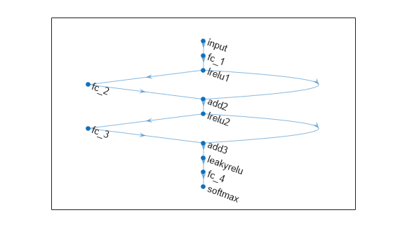
Define a neural network architecture with these characteristics:
A feature input layer with an input size that matches the number of predictors.
Three fully connected layers followed by leaky ReLU layers, connected in series, where the fully connected layers have output sizes of 16, and addition layers after the second and third fully connected layers.
Skip connections around the second and third fully connected layers using the addition layers.
A final fully connected layer with an output size that matches the number of classes followed by a softmax layer.
inputSize = size(XTrain,2);
outputSize = numel(unique(YTrain));

net = dlnetwork;

layers = [
    featureInputLayer(inputSize)
    fullyConnectedLayer(30)
    leakyReluLayer(Name="lrelu1")

    fullyConnectedLayer(30)

    additionLayer(2,Name="add2")
    leakyReluLayer(Name="lrelu2")

    fullyConnectedLayer(30)
    additionLayer(2,Name="add3")
    leakyReluLayer

    fullyConnectedLayer(outputSize)
    softmaxLayer];

net = addLayers(net,layers);
net = connectLayers(net,"lrelu1","add2/in2");
net = connectLayers(net,"lrelu2","add3/in2");
Visualize the neural network architecture in a plot.
figure
plot(net)
Train a neural network classifier.
Mdl = fitcnet(XTrain,YTrain,Network=net,Standardize=true)
Mdl =
  ClassificationNeuralNetwork
             ResponseName: 'Y'
    CategoricalPredictors: []
               ClassNames: {'b'  'g'}
           ScoreTransform: 'none'
          NumObservations: 246
               LayerSizes: []
              Activations: ''
    OutputLayerActivation: ''
                   Solver: 'LBFGS'
          ConvergenceInfo: [1×1 struct]
          TrainingHistory: [30×7 table]

  View network information using dlnetwork.


  Properties, Methods
To estimate the performance of the trained classifier, compute the test set classification error.
testError = loss(Mdl,XTest,YTest, ...
    LossFun="classiferror")
testError =
0.0774
At each iteration of the training process, compute the validation loss of the neural network. Stop the training process early if the validation loss reaches a reasonable minimum.
Load the patients data set. Create a table from the data set. Each row corresponds to one patient, and each column corresponds to a diagnostic variable. Use the Smoker variable as the response variable, and the rest of the variables as predictors.
load patients
tbl = table(Diastolic,Systolic,Gender,Height,Weight,Age,Smoker);
Separate the data into a training set tblTrain and a validation set tblValidation by using a stratified holdout partition. The software reserves approximately 30% of the observations for the validation data set and uses the rest of the observations for the training data set.
rng("default") % For reproducibility of the partition
c = cvpartition(tbl.Smoker,"Holdout",0.30);
trainingIndices = training(c);
validationIndices = test(c);
tblTrain = tbl(trainingIndices,:);
tblValidation = tbl(validationIndices,:);
Train a neural network classifier by using the training set. Specify the Smoker column of tblTrain as the response variable. Evaluate the model at each iteration by using the validation set. Specify to display the training information at each iteration by using the Verbose name-value argument. By default, the training process ends early if the validation cross-entropy loss is greater than or equal to the minimum validation cross-entropy loss computed so far, six times in a row. To change the number of times the validation loss is allowed to be greater than or equal to the minimum, specify the ValidationPatience name-value argument.
Mdl = fitcnet(tblTrain,"Smoker", ...
    "ValidationData",tblValidation, ...
    "Verbose",1);
|==========================================================================================|
| Iteration  | Train Loss | Gradient   | Step       | Iteration  | Validation | Validation |
|            |            |            |            | Time (sec) | Loss       | Checks     |
|==========================================================================================|
|           1|    2.602935|   26.866935|    0.262009|    0.021430|    2.793048|           0|
|           2|    1.470816|   42.594723|    0.058323|    0.004188|    1.247046|           0|
|           3|    1.299292|   25.854432|    0.034910|    0.002086|    1.507857|           1|
|           4|    0.710465|   11.629107|    0.013616|    0.002767|    0.889157|           0|
|           5|    0.647783|    2.561740|    0.005753|    0.005871|    0.766728|           0|
|           6|    0.645541|    0.681579|    0.001000|    0.000919|    0.776072|           1|
|           7|    0.639611|    1.544692|    0.007013|    0.005747|    0.776320|           2|
|           8|    0.604189|    5.045676|    0.064190|    0.000217|    0.744919|           0|
|           9|    0.565364|    5.851552|    0.068845|    0.000233|    0.694226|           0|
|          10|    0.391994|    8.377717|    0.560480|    0.000161|    0.425466|           0|
|==========================================================================================|
| Iteration  | Train Loss | Gradient   | Step       | Iteration  | Validation | Validation |
|            |            |            |            | Time (sec) | Loss       | Checks     |
|==========================================================================================|
|          11|    0.383843|    0.630246|    0.110270|    0.000763|    0.428487|           1|
|          12|    0.369289|    2.404750|    0.084395|    0.000318|    0.405728|           0|
|          13|    0.357839|    6.220679|    0.199197|    0.000255|    0.378480|           0|
|          14|    0.344974|    2.752717|    0.029013|    0.000186|    0.367279|           0|
|          15|    0.333747|    0.711398|    0.074513|    0.000911|    0.348499|           0|
|          16|    0.327763|    0.804818|    0.122178|    0.000301|    0.330237|           0|
|          17|    0.327702|    0.778169|    0.009810|    0.000166|    0.329095|           0|
|          18|    0.327277|    0.020615|    0.004377|    0.000159|    0.329141|           1|
|          19|    0.327273|    0.010018|    0.003313|    0.000157|    0.328773|           0|
|          20|    0.327268|    0.019497|    0.000805|    0.000320|    0.328831|           1|
|==========================================================================================|
| Iteration  | Train Loss | Gradient   | Step       | Iteration  | Validation | Validation |
|            |            |            |            | Time (sec) | Loss       | Checks     |
|==========================================================================================|
|          21|    0.327228|    0.113983|    0.005397|    0.007385|    0.329085|           2|
|          22|    0.327138|    0.240166|    0.012159|    0.001329|    0.329406|           3|
|          23|    0.326865|    0.428912|    0.036841|    0.000160|    0.329952|           4|
|          24|    0.325797|    0.255227|    0.139585|    0.000175|    0.331246|           5|
|          25|    0.325181|    0.758050|    0.135868|    0.000395|    0.332035|           6|
|==========================================================================================|
Create a plot that compares the training cross-entropy loss and the validation cross-entropy loss at each iteration. By default, fitcnet stores the loss information inside the TrainingHistory property of the object Mdl. You can access this information by using dot notation.
iteration = Mdl.TrainingHistory.Iteration;
trainLosses = Mdl.TrainingHistory.TrainingLoss;
valLosses = Mdl.TrainingHistory.ValidationLoss;

plot(iteration,trainLosses,iteration,valLosses)
legend(["Training","Validation"])
xlabel("Iteration")
ylabel("Cross-Entropy Loss")
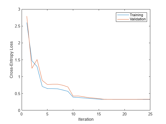
Check the iteration that corresponds to the minimum validation loss. The final returned model Mdl is the model trained at this iteration.
[~,minIdx] = min(valLosses);
iteration(minIdx)
ans =
19
Assess the cross-validation loss of neural network models with different regularization strengths, and choose the regularization strength corresponding to the best performing model.
Read the sample file CreditRating_Historical.dat into a table. The predictor data consists of financial ratios and industry sector information for a list of corporate customers. The response variable consists of credit ratings assigned by a rating agency. Preview the first few rows of the data set.
creditrating = readtable("CreditRating_Historical.dat");
head(creditrating)
ID WC_TA RE_TA EBIT_TA MVE_BVTD S_TA Industry Rating
_____ ______ ______ _______ ________ _____ ________ _______
62394 0.013 0.104 0.036 0.447 0.142 3 {'BB' }
48608 0.232 0.335 0.062 1.969 0.281 8 {'A' }
42444 0.311 0.367 0.074 1.935 0.366 1 {'A' }
48631 0.194 0.263 0.062 1.017 0.228 4 {'BBB'}
43768 0.121 0.413 0.057 3.647 0.466 12 {'AAA'}
39255 -0.117 -0.799 0.01 0.179 0.082 4 {'CCC'}
62236 0.087 0.158 0.049 0.816 0.324 2 {'BBB'}
39354 0.005 0.181 0.034 2.597 0.388 7 {'AA' }
Because each value in the ID variable is a unique customer ID, that is, length(unique(creditrating.ID)) is equal to the number of observations in creditrating, the ID variable is a poor predictor. Remove the ID variable from the table, and convert the Industry variable to a categorical variable.
creditrating = removevars(creditrating,"ID");
creditrating.Industry = categorical(creditrating.Industry);
Convert the Rating response variable to a categorical variable.
creditrating.Rating = categorical(creditrating.Rating, ...
    ["AAA","AA","A","BBB","BB","B","CCC"]);
Create a cvpartition object for stratified 5-fold cross-validation. cvp partitions the data into five folds, where each fold has roughly the same proportions of different credit ratings. Set the random seed to the default value for reproducibility of the partition.
rng("default")
cvp = cvpartition(creditrating.Rating,"KFold",5);
Compute the cross-validation classification error for neural network classifiers with different regularization strengths. Try regularization strengths on the order of 1/n, where n is the number of observations. Specify to standardize the data before training the neural network models.
1/size(creditrating,1)
ans = 2.5432e-04
lambda = (0:0.5:5)*1e-4;
cvloss = zeros(length(lambda),1);

for i = 1:length(lambda)
    cvMdl = fitcnet(creditrating,"Rating","Lambda",lambda(i), ...
        "CVPartition",cvp,"Standardize",true);
    cvloss(i) = kfoldLoss(cvMdl,"LossFun","classiferror");
end
Plot the results. Find the regularization strength corresponding to the lowest cross-validation classification error.
plot(lambda,cvloss)
xlabel("Regularization Strength")
ylabel("Cross-Validation Loss")
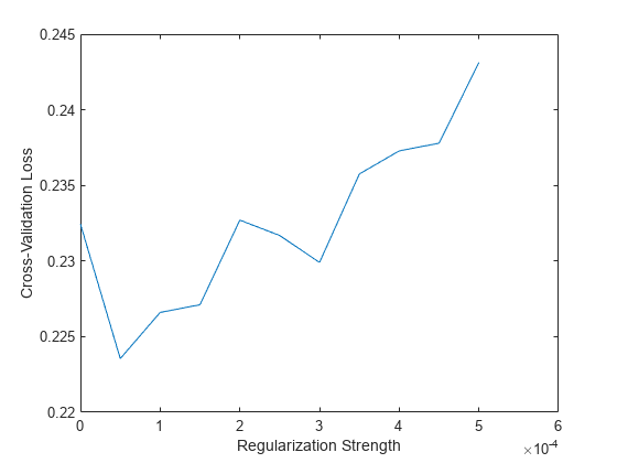
[~,idx] = min(cvloss);
bestLambda = lambda(idx)
bestLambda = 5.0000e-05
Train a neural network classifier using the bestLambda regularization strength.
Mdl = fitcnet(creditrating,"Rating","Lambda",bestLambda, ...
    "Standardize",true)
Mdl =
  ClassificationNeuralNetwork
           PredictorNames: {'WC_TA'  'RE_TA'  'EBIT_TA'  'MVE_BVTD'  'S_TA'  'Industry'}
             ResponseName: 'Rating'
    CategoricalPredictors: 6
               ClassNames: [AAA    AA    A    BBB    BB    B    CCC]
           ScoreTransform: 'none'
          NumObservations: 3932
               LayerSizes: 10
              Activations: 'relu'
    OutputLayerActivation: 'softmax'
                   Solver: 'LBFGS'
          ConvergenceInfo: [1×1 struct]
          TrainingHistory: [1000×7 table]


  Properties, Methods
Train a neural network classifier using the OptimizeHyperparameters argument to improve the resulting classifier. Using this argument causes fitcnet to minimize cross-validation loss over some problem hyperparameters using Bayesian optimization.
Read the sample file CreditRating_Historical.dat into a table. The predictor data consists of financial ratios and industry sector information for a list of corporate customers. The response variable consists of credit ratings assigned by a rating agency. Preview the first few rows of the data set.
creditrating = readtable("CreditRating_Historical.dat");
head(creditrating)
ID WC_TA RE_TA EBIT_TA MVE_BVTD S_TA Industry Rating
_____ ______ ______ _______ ________ _____ ________ _______
62394 0.013 0.104 0.036 0.447 0.142 3 {'BB' }
48608 0.232 0.335 0.062 1.969 0.281 8 {'A' }
42444 0.311 0.367 0.074 1.935 0.366 1 {'A' }
48631 0.194 0.263 0.062 1.017 0.228 4 {'BBB'}
43768 0.121 0.413 0.057 3.647 0.466 12 {'AAA'}
39255 -0.117 -0.799 0.01 0.179 0.082 4 {'CCC'}
62236 0.087 0.158 0.049 0.816 0.324 2 {'BBB'}
39354 0.005 0.181 0.034 2.597 0.388 7 {'AA' }
Because each value in the ID variable is a unique customer ID, that is, length(unique(creditrating.ID)) is equal to the number of observations in creditrating, the ID variable is a poor predictor. Remove the ID variable from the table, and convert the Industry variable to a categorical variable.
creditrating = removevars(creditrating,"ID");
creditrating.Industry = categorical(creditrating.Industry);
Convert the Rating response variable to a categorical variable.
creditrating.Rating = categorical(creditrating.Rating, ...
    ["AAA","AA","A","BBB","BB","B","CCC"]);
Partition the data into training and test sets. Use approximately 80% of the observations to train a neural network model, and 20% of the observations to test the performance of the trained model on new data. Use cvpartition to partition the data.
rng("default") % For reproducibility of the partition
c = cvpartition(creditrating.Rating,Holdout=0.20);

trainingIndices = training(c);
testIndices = test(c);

creditTrain = creditrating(trainingIndices,:);
creditTest = creditrating(testIndices,:);
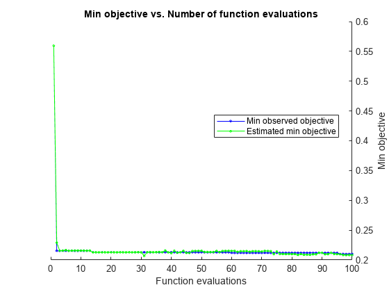
Train a neural network classifier by passing the training data creditTrain to the fitcnet function, and include the OptimizeHyperparameters argument. For reproducibility, set the AcquisitionFunctionName to "expected-improvement-plus" in a HyperparameterOptimizationOptions object. To attempt to get a better solution, set the number of optimization steps to 100 instead of the default 30. fitcnet performs Bayesian optimization by default. To use grid search or random search, set the Optimizer value in HyperparameterOptimizationOptions.
rng("default") % For reproducibility
hpoOptions = hyperparameterOptimizationOptions(AcquisitionFunctionName="expected-improvement-plus", ...
    MaxObjectiveEvaluations=100);
Mdl = fitcnet(creditTrain,"Rating",OptimizeHyperparameters="auto", ...
    HyperparameterOptimizationOptions=hpoOptions)
|============================================================================================================================================|
| Iter | Eval | Objective | Objective | BestSoFar | BestSoFar | Activations | Standardize | Lambda | LayerSizes |
| | result | | runtime | (observed) | (estim.) | | | | |
|============================================================================================================================================|
| 1 | Best | 0.55944 | 3.228 | 0.55944 | 0.55944 | none | true | 0.05834 | 3 |
| 2 | Best | 0.21424 | 11.121 | 0.21424 | 0.22797 | relu | true | 5.0811e-08 | [ 1 25] |
| 3 | Accept | 0.74189 | 0.68788 | 0.21424 | 0.21448 | sigmoid | true | 0.57986 | 126 |
| 4 | Accept | 0.4501 | 0.96922 | 0.21424 | 0.21438 | tanh | false | 0.018683 | 10 |
| 5 | Accept | 0.74189 | 0.67572 | 0.21424 | 0.2357 | relu | true | 0.87757 | [ 84 278] |
| 6 | Best | 0.21297 | 11.293 | 0.21297 | 0.21363 | relu | true | 8.9142e-08 | [ 1 22] |
| 7 | Accept | 0.47139 | 0.74146 | 0.21297 | 0.21363 | relu | true | 0.0059137 | 1 |
| 8 | Accept | 0.63318 | 2.4328 | 0.21297 | 0.21363 | relu | true | 3.0482e-07 | [ 1 1 1] |
| 9 | Best | 0.21233 | 7.9275 | 0.21233 | 0.21362 | tanh | true | 9.2841e-05 | [ 1 3] |
| 10 | Accept | 0.21297 | 14.363 | 0.21233 | 0.21362 | tanh | false | 9.6057e-05 | [ 1 29] |
| 11 | Accept | 0.45868 | 0.39227 | 0.21233 | 0.2124 | tanh | false | 0.022609 | 13 |
| 12 | Accept | 0.22155 | 39.202 | 0.21233 | 0.21235 | tanh | true | 8.582e-07 | [ 3 142] |
| 13 | Accept | 0.32645 | 34.129 | 0.21233 | 0.21236 | tanh | true | 0.00011739 | [152 1] |
| 14 | Accept | 0.226 | 9.8645 | 0.21233 | 0.21363 | tanh | false | 1.6285e-07 | [ 5 6] |
| 15 | Accept | 0.74189 | 0.78611 | 0.21233 | 0.21363 | tanh | false | 0.064854 | [300 19] |
| 16 | Accept | 0.74189 | 0.15971 | 0.21233 | 0.21236 | tanh | false | 20.576 | [ 2 1] |
| 17 | Accept | 0.21583 | 12.747 | 0.21233 | 0.21236 | tanh | false | 3.5661e-06 | [ 1 20] |
| 18 | Accept | 0.30006 | 70.791 | 0.21233 | 0.21237 | relu | true | 3.0202e-08 | [ 63 272] |
| 19 | Accept | 0.23935 | 48.639 | 0.21233 | 0.21239 | tanh | false | 1.3422e-06 | [178 3] |
| 20 | Accept | 0.21488 | 8.7877 | 0.21233 | 0.21244 | tanh | true | 8.4864e-06 | [ 1 3] |
|============================================================================================================================================|
| Iter | Eval | Objective | Objective | BestSoFar | BestSoFar | Activations | Standardize | Lambda | LayerSizes |
| | result | | runtime | (observed) | (estim.) | | | | |
|============================================================================================================================================|
| 21 | Accept | 0.21647 | 9.2742 | 0.21233 | 0.21243 | tanh | true | 6.2116e-09 | [ 1 5] |
| 22 | Accept | 0.74189 | 0.14105 | 0.21233 | 0.21249 | tanh | true | 0.32388 | [ 1 5] |
| 23 | Accept | 0.29911 | 54.688 | 0.21233 | 0.2125 | tanh | true | 1.3072e-08 | [279 243] |
| 24 | Accept | 0.2171 | 10.036 | 0.21233 | 0.21253 | tanh | true | 7.0461e-08 | [ 1 11] |
| 25 | Accept | 0.22759 | 59.969 | 0.21233 | 0.21255 | tanh | false | 3.2952e-09 | [265 2] |
| 26 | Accept | 0.21551 | 50.424 | 0.21233 | 0.21257 | tanh | false | 3.2467e-09 | [ 1 219] |
| 27 | Accept | 0.21297 | 7.3527 | 0.21233 | 0.21259 | tanh | false | 4.9649e-07 | 1 |
| 28 | Accept | 0.21456 | 6.4024 | 0.21233 | 0.2126 | relu | true | 3.4266e-08 | 1 |
| 29 | Accept | 0.21583 | 7.9678 | 0.21233 | 0.2126 | tanh | false | 3.198e-09 | 4 |
| 30 | Accept | 0.21329 | 6.7581 | 0.21233 | 0.2126 | tanh | true | 2.1844e-07 | 1 |
| 31 | Accept | 0.21456 | 6.7172 | 0.21233 | 0.21261 | tanh | true | 3.491e-09 | 1 |
| 32 | Accept | 0.21742 | 6.6492 | 0.21233 | 0.21262 | relu | true | 1.079e-06 | 1 |
| 33 | Accept | 0.28894 | 58.848 | 0.21233 | 0.21261 | tanh | false | 6.3869e-08 | 295 |
| 34 | Accept | 0.22441 | 15.532 | 0.21233 | 0.21261 | tanh | false | 1.2882e-08 | [ 18 1 8] |
| 35 | Accept | 0.21678 | 11.457 | 0.21233 | 0.21261 | tanh | false | 4.4949e-06 | [ 1 10 4] |
| 36 | Accept | 0.21424 | 87.852 | 0.21233 | 0.2126 | tanh | true | 5.3964e-06 | [ 1 247 86] |
| 37 | Accept | 0.21869 | 58.217 | 0.21233 | 0.2126 | tanh | true | 5.0039e-09 | [ 1 148 53] |
| 38 | Accept | 0.21996 | 90.511 | 0.21233 | 0.2126 | tanh | false | 5.4247e-07 | [286 1 150] |
| 39 | Accept | 0.23872 | 5.212 | 0.21233 | 0.21263 | tanh | false | 1.7157e-05 | 1 |
| 40 | Accept | 0.2136 | 47.562 | 0.21233 | 0.21264 | tanh | true | 1.8512e-07 | [ 1 1 220] |
|============================================================================================================================================|
| Iter | Eval | Objective | Objective | BestSoFar | BestSoFar | Activations | Standardize | Lambda | LayerSizes |
| | result | | runtime | (observed) | (estim.) | | | | |
|============================================================================================================================================|
| 41 | Accept | 0.26383 | 3.2043 | 0.21233 | 0.21274 | tanh | true | 3.1114e-05 | 1 |
| 42 | Accept | 0.2171 | 7.0619 | 0.21233 | 0.21264 | relu | false | 3.3305e-09 | 1 |
| 43 | Accept | 0.26923 | 24.412 | 0.21233 | 0.21264 | relu | false | 2.2917e-06 | 100 |
| 44 | Accept | 0.28322 | 57.67 | 0.21233 | 0.21264 | relu | false | 3.2127e-09 | [288 48] |
| 45 | Accept | 0.23045 | 11.199 | 0.21233 | 0.21263 | relu | false | 1.5945e-05 | [ 1 14 11] |
| 46 | Accept | 0.21392 | 21.227 | 0.21233 | 0.21269 | relu | false | 5.1866e-07 | [ 1 56] |
| 47 | Accept | 0.74189 | 0.16414 | 0.21233 | 0.2126 | relu | false | 0.0048979 | [ 1 1] |
| 48 | Accept | 0.21933 | 49.762 | 0.21233 | 0.2126 | relu | false | 1.4139e-07 | [ 1 16 231] |
| 49 | Accept | 0.27241 | 81.412 | 0.21233 | 0.2126 | relu | false | 1.3403e-06 | [288 102 32] |
| 50 | Accept | 0.21837 | 7.2282 | 0.21233 | 0.2126 | relu | false | 5.8044e-08 | 1 |
| 51 | Accept | 0.29053 | 49.915 | 0.21233 | 0.21259 | relu | false | 1.8365e-08 | 299 |
| 52 | Accept | 0.21551 | 39.82 | 0.21233 | 0.2126 | relu | false | 1.167e-08 | [ 1 209] |
| 53 | Accept | 0.21456 | 13.05 | 0.21233 | 0.21259 | sigmoid | false | 3.4117e-09 | [ 2 20] |
| 54 | Accept | 0.21551 | 25.437 | 0.21233 | 0.21259 | sigmoid | false | 5.4928e-07 | [ 2 1 61] |
| 55 | Accept | 0.2314 | 58.394 | 0.21233 | 0.21259 | sigmoid | false | 9.179e-07 | [265 5] |
| 56 | Accept | 0.23458 | 64.653 | 0.21233 | 0.21259 | sigmoid | false | 3.6282e-09 | [289 10 5] |
| 57 | Accept | 0.74189 | 1.1248 | 0.21233 | 0.21258 | sigmoid | false | 0.0041382 | [ 1 4 102] |
| 58 | Accept | 0.21551 | 40.952 | 0.21233 | 0.21259 | sigmoid | false | 8.6375e-08 | [ 1 202] |
| 59 | Accept | 0.24952 | 52.29 | 0.21233 | 0.21259 | sigmoid | false | 7.0357e-09 | 276 |
| 60 | Accept | 0.23204 | 70.117 | 0.21233 | 0.21259 | sigmoid | false | 1.2977e-07 | [284 6 34] |
|============================================================================================================================================|
| Iter | Eval | Objective | Objective | BestSoFar | BestSoFar | Activations | Standardize | Lambda | LayerSizes |
| | result | | runtime | (observed) | (estim.) | | | | |
|============================================================================================================================================|
| 61 | Accept | 0.22123 | 14.019 | 0.21233 | 0.21259 | sigmoid | false | 2.0622e-08 | [ 1 17 3] |
| 62 | Accept | 0.21742 | 29.239 | 0.21233 | 0.21258 | none | false | 3.5451e-09 | [ 4 209] |
| 63 | Accept | 0.2206 | 29.504 | 0.21233 | 0.21258 | none | false | 5.8688e-07 | 189 |
| 64 | Accept | 0.2206 | 28.077 | 0.21233 | 0.21258 | none | false | 1.2001e-06 | [111 17 16] |
| 65 | Accept | 0.21488 | 7.8422 | 0.21233 | 0.21258 | none | false | 7.5066e-07 | [ 1 12] |
| 66 | Accept | 0.22123 | 5.4097 | 0.21233 | 0.21258 | none | false | 0.001714 | [263 2] |
| 67 | Accept | 0.22854 | 0.85958 | 0.21233 | 0.21258 | none | false | 0.00034066 | 1 |
| 68 | Accept | 0.74189 | 0.32181 | 0.21233 | 0.21258 | none | false | 2.3034 | 296 |
| 69 | Accept | 0.21996 | 28.273 | 0.21233 | 0.21258 | none | false | 4.7355e-05 | [211 18] |
| 70 | Accept | 0.21551 | 3.4669 | 0.21233 | 0.21259 | none | false | 0.00066664 | [ 1 45 6] |
| 71 | Accept | 0.21996 | 36.461 | 0.21233 | 0.21259 | none | false | 4.3257e-09 | [267 12 6] |
| 72 | Accept | 0.21583 | 2.1001 | 0.21233 | 0.21259 | none | false | 0.00032204 | [ 1 6] |
| 73 | Accept | 0.21996 | 58.211 | 0.21233 | 0.21259 | none | false | 4.8158e-08 | [285 73] |
| 74 | Accept | 0.21488 | 7.0801 | 0.21233 | 0.2126 | none | false | 3.6333e-08 | [ 1 31 38] |
| 75 | Accept | 0.21488 | 5.2708 | 0.21233 | 0.2126 | none | false | 8.7551e-09 | 1 |
| 76 | Accept | 0.21964 | 9.6975 | 0.21233 | 0.2126 | none | true | 4.0779e-09 | [ 5 2 23] |
| 77 | Accept | 0.21996 | 9.2044 | 0.21233 | 0.21259 | none | true | 3.2393e-09 | 150 |
| 78 | Accept | 0.21996 | 23.793 | 0.21233 | 0.21259 | none | true | 1.3751e-07 | [298 9] |
| 79 | Accept | 0.21488 | 3.1085 | 0.21233 | 0.21261 | none | true | 3.26e-09 | [ 1 2] |
| 80 | Accept | 0.22028 | 27.002 | 0.21233 | 0.2126 | none | true | 4.1203e-09 | [286 158] |
|============================================================================================================================================|
| Iter | Eval | Objective | Objective | BestSoFar | BestSoFar | Activations | Standardize | Lambda | LayerSizes |
| | result | | runtime | (observed) | (estim.) | | | | |
|============================================================================================================================================|
| 81 | Accept | 0.21488 | 11.484 | 0.21233 | 0.21264 | none | true | 6.0989e-07 | [ 1 36 31] |
| 82 | Accept | 0.21456 | 3.8323 | 0.21233 | 0.21264 | none | true | 1.2566e-07 | 1 |
| 83 | Accept | 0.21933 | 5.1454 | 0.21233 | 0.21269 | none | false | 0.00014314 | [ 15 1 36] |
| 84 | Accept | 0.21329 | 43.462 | 0.21233 | 0.21249 | tanh | true | 7.3541e-05 | [ 1 194] |
| 85 | Accept | 0.21583 | 10.828 | 0.21233 | 0.21249 | sigmoid | true | 3.4114e-09 | [ 1 7 2] |
| 86 | Accept | 0.31182 | 53.861 | 0.21233 | 0.21249 | sigmoid | true | 3.218e-09 | 263 |
| 87 | Accept | 0.3042 | 89.634 | 0.21233 | 0.21247 | sigmoid | true | 3.5681e-07 | [278 58 57] |
| 88 | Accept | 0.29911 | 125.19 | 0.21233 | 0.21246 | sigmoid | true | 3.2323e-09 | [273 224 6] |
| 89 | Accept | 0.21488 | 21.777 | 0.21233 | 0.21245 | sigmoid | true | 3.1838e-08 | [ 1 63] |
| 90 | Accept | 0.21488 | 1.8753 | 0.21233 | 0.21244 | none | true | 5.5242e-08 | [ 1 28 11] |
| 91 | Accept | 0.21647 | 3.2709 | 0.21233 | 0.21244 | none | false | 6.1228e-06 | 1 |
| 92 | Accept | 0.21933 | 44.399 | 0.21233 | 0.21243 | none | true | 5.208e-05 | [292 29 26] |
| 93 | Accept | 0.21297 | 37.538 | 0.21233 | 0.21244 | none | true | 1.49e-06 | [248 7 1] |
| 94 | Accept | 0.28862 | 8.5087 | 0.21233 | 0.21246 | sigmoid | true | 3.2426e-09 | [ 1 2] |
| 95 | Accept | 0.21424 | 7.0729 | 0.21233 | 0.21245 | sigmoid | true | 5.8982e-07 | 1 |
| 96 | Accept | 0.23617 | 9.5403 | 0.21233 | 0.21245 | sigmoid | true | 3.3336e-08 | [ 1 1 2] |
| 97 | Accept | 0.21488 | 43.813 | 0.21233 | 0.21244 | sigmoid | true | 5.4613e-07 | [ 1 264] |
| 98 | Accept | 0.21424 | 6.7632 | 0.21233 | 0.21244 | none | true | 7.1488e-06 | [ 1 3] |
| 99 | Accept | 0.21996 | 21.803 | 0.21233 | 0.21244 | none | true | 3.7238e-06 | 230 |
| 100 | Accept | 0.21519 | 7.0249 | 0.21233 | 0.21243 | sigmoid | true | 8.1517e-08 | 1 |
__________________________________________________________
Optimization completed.
MaxObjectiveEvaluations of 100 reached.
Total function evaluations: 100
Total elapsed time: 2499.2017 seconds
Total objective function evaluation time: 2445.3645
Best observed feasible point:
Activations Standardize Lambda LayerSizes
___________ ___________ __________ __________
tanh true 9.2841e-05 1 3
Observed objective function value = 0.21233
Estimated objective function value = 0.21344
Function evaluation time = 7.9275
Best estimated feasible point (according to models):
Activations Standardize Lambda LayerSizes
___________ ___________ __________ __________
tanh true 7.3541e-05 1 194
Estimated objective function value = 0.21243
Estimated function evaluation time = 34.5594
Mdl =
  ClassificationNeuralNetwork
                       PredictorNames: {'WC_TA'  'RE_TA'  'EBIT_TA'  'MVE_BVTD'  'S_TA'  'Industry'}
                         ResponseName: 'Rating'
                CategoricalPredictors: 6
                           ClassNames: [AAA    AA    A    BBB    BB    B    CCC]
                       ScoreTransform: 'none'
                      NumObservations: 3146
    HyperparameterOptimizationResults: [1×1 classreg.learning.paramoptim.SupervisedLearningBayesianOptimization]
                           LayerSizes: [1 194]
                          Activations: 'tanh'
                OutputLayerActivation: 'softmax'
                               Solver: 'LBFGS'
                      ConvergenceInfo: [1×1 struct]
                      TrainingHistory: [1000×7 table]


  Properties, Methods
The trained classifier Mdl corresponds to the best estimated feasible point and uses the same hyperparameter values for Activations, Standardize, Lambda, and LayerSizes.
Find the hyperparameter values used to train Mdl by using the bestPoint function. By default, bestPoint uses the same best point criterion used by fitcnet during the hyperparameter optimization ("min-visited-upper-confidence-interval"). In general, fit functions determine the best hyperparameter values based on the "min-visited-upper-confidence-interval" criterion (instead of the "min-observed" criterion) to avoid overfitting to noise in the data set.
bestEstimatedPoint = bestPoint(Mdl.HyperparameterOptimizationResults)
bestEstimatedPoint=1×7 table
    NumLayers    Activations    Standardize      Lambda      Layer_1_Size    Layer_2_Size    Layer_3_Size
    _________    ___________    ___________    __________    ____________    ____________    ____________

        2           tanh           true        7.3541e-05         1              194             NaN
Verify that the results match the properties of Mdl. Note that the Mu and Sigma properties of a ClassificationNeuralNetwork object are nonempty when the neural network model uses standardization.
modelProperties = table(length(Mdl.LayerSizes), ...
    string(Mdl.Activations), ...
    struct(Means=Mdl.Mu,StandardDeviations=Mdl.Sigma), ...
    Mdl.ModelParameters.Lambda,Mdl.LayerSizes, ...
    VariableNames=["NumLayers","Activations","Standardize", ...
    "Lambda","LayerSizes"])
modelProperties=1×5 table
    NumLayers    Activations    Standardize      Lambda      LayerSizes
    _________    ___________    ___________    __________    __________

        2          "tanh"       1×1 struct     7.3541e-05     1    194
modelProperties.Standardize
ans = struct with fields:
                 Means: [0.1392 0.2053 0.0513 2.0712 0.3068 0 0 0 0 0 0 0 0 0 0 0 0]
    StandardDeviations: [0.1762 0.3453 0.0311 4.2033 0.2555 1 1 1 1 1 1 1 1 1 1 1 1]
Find the classification accuracy of the model on the test data set. Visualize the results by using a confusion matrix.
modelAccuracy = 1 - loss(Mdl,creditTest,"Rating", ...
    LossFun="classiferror")
modelAccuracy =
0.8015
confusionchart(creditTest.Rating,predict(Mdl,creditTest))
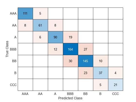
The model has all predicted classes within one unit of the true classes, meaning all predictions are off by no more than one rating.
Train a neural network classifier using the OptimizeHyperparameters argument to improve the resulting classification accuracy. Use the hyperparameters function to specify larger-than-default values for the number of layers used and the layer size range.
Read the sample file CreditRating_Historical.dat into a table. The predictor data consists of financial ratios and industry sector information for a list of corporate customers. The response variable consists of credit ratings assigned by a rating agency.
creditrating = readtable("CreditRating_Historical.dat");Because each value in the ID variable is a unique customer ID, that is, length(unique(creditrating.ID)) is equal to the number of observations in creditrating, the ID variable is a poor predictor. Remove the ID variable from the table, and convert the Industry variable to a categorical variable.
creditrating = removevars(creditrating,"ID");
creditrating.Industry = categorical(creditrating.Industry);
Convert the Rating response variable to a categorical variable.
creditrating.Rating = categorical(creditrating.Rating, ...
    ["AAA","AA","A","BBB","BB","B","CCC"]);
Partition the data into training and test sets. Use approximately 80% of the observations to train a neural network model, and 20% of the observations to test the performance of the trained model on new data. Use cvpartition to partition the data.
rng("default") % For reproducibility of the partition
c = cvpartition(creditrating.Rating,Holdout=0.20);
trainingIndices = training(c); % Indices for the training set
testIndices = test(c); % Indices for the test set
creditTrain = creditrating(trainingIndices,:);
creditTest = creditrating(testIndices,:);
List the hyperparameters available for this problem of fitting the Rating response.
params = hyperparameters("fitcnet",creditTrain,"Rating");
for ii = 1:length(params)
    disp(ii);disp(params(ii))
end
     1

  optimizableVariable with properties:

         Name: 'NumLayers'
        Range: [1 3]
         Type: 'integer'
    Transform: 'none'
     Optimize: 1

     2

  optimizableVariable with properties:

         Name: 'Activations'
        Range: {'relu'  'tanh'  'sigmoid'  'none'}
         Type: 'categorical'
    Transform: 'none'
     Optimize: 1

     3

  optimizableVariable with properties:

         Name: 'Standardize'
        Range: {'true'  'false'}
         Type: 'categorical'
    Transform: 'none'
     Optimize: 1

     4

  optimizableVariable with properties:

         Name: 'Lambda'
        Range: [3.1786e-09 31.7864]
         Type: 'real'
    Transform: 'log'
     Optimize: 1

     5

  optimizableVariable with properties:

         Name: 'LayerWeightsInitializer'
        Range: {'glorot'  'he'}
         Type: 'categorical'
    Transform: 'none'
     Optimize: 0

     6

  optimizableVariable with properties:

         Name: 'LayerBiasesInitializer'
        Range: {'zeros'  'ones'}
         Type: 'categorical'
    Transform: 'none'
     Optimize: 0

     7

  optimizableVariable with properties:

         Name: 'Layer_1_Size'
        Range: [1 300]
         Type: 'integer'
    Transform: 'log'
     Optimize: 1

     8

  optimizableVariable with properties:

         Name: 'Layer_2_Size'
        Range: [1 300]
         Type: 'integer'
    Transform: 'log'
     Optimize: 1

     9

  optimizableVariable with properties:

         Name: 'Layer_3_Size'
        Range: [1 300]
         Type: 'integer'
    Transform: 'log'
     Optimize: 1

    10

  optimizableVariable with properties:

         Name: 'Layer_4_Size'
        Range: [1 300]
         Type: 'integer'
    Transform: 'log'
     Optimize: 0

    11

  optimizableVariable with properties:

         Name: 'Layer_5_Size'
        Range: [1 300]
         Type: 'integer'
    Transform: 'log'
     Optimize: 0
To try more layers than the default of 1 through 3, set the range of NumLayers (optimizable variable 1) to its maximum allowable size, [1 5]. Also, set Layer_4_Size and Layer_5_Size (optimizable variables 10 and 11, respectively) to be optimized.
params(1).Range = [1 5];
params(10).Optimize = true;
params(11).Optimize = true;
Set the range of all layer sizes (optimizable variables 7 through 11) to [1 400] instead of the default [1 300].
for ii = 7:11
    params(ii).Range = [1 400];
end
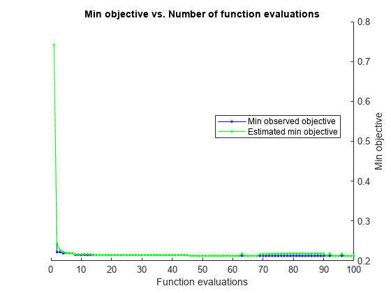
Train a neural network classifier by passing the training data creditTrain to the fitcnet function, and include the OptimizeHyperparameters argument set to params. For reproducibility, set the AcquisitionFunctionName to "expected-improvement-plus" in a HyperparameterOptimizationOptions structure. To attempt to get a better solution, set the number of optimization steps to 100 instead of the default 30.
rng("default") % For reproducibility
Mdl = fitcnet(creditTrain,"Rating",OptimizeHyperparameters=params, ...
    HyperparameterOptimizationOptions= ...
    struct(AcquisitionFunctionName="expected-improvement-plus", ...
    MaxObjectiveEvaluations=100))
|============================================================================================================================================|
| Iter | Eval | Objective | Objective | BestSoFar | BestSoFar | Activations | Standardize | Lambda | LayerSizes |
| | result | | runtime | (observed) | (estim.) | | | | |
|============================================================================================================================================|
| 1 | Best | 0.74189 | 2.9742 | 0.74189 | 0.74189 | sigmoid | true | 0.68961 | [104 1 5 3 1] |
| 2 | Best | 0.22155 | 82.971 | 0.22155 | 0.24224 | relu | true | 0.00058564 | [ 38 208 162] |
| 3 | Accept | 0.64018 | 15.831 | 0.22155 | 0.22597 | sigmoid | true | 1.9768e-06 | [ 1 25 1 287 7] |
| 4 | Best | 0.22028 | 38.683 | 0.22028 | 0.22381 | none | false | 1.3353e-06 | 320 |
| 5 | Accept | 0.74189 | 0.31099 | 0.22028 | 0.22031 | relu | true | 2.7056 | [ 1 2 1] |
| 6 | Accept | 0.30356 | 111.92 | 0.22028 | 0.22031 | relu | true | 1.0503e-06 | [301 31 400] |
| 7 | Accept | 0.68722 | 5.7457 | 0.22028 | 0.22031 | relu | true | 0.0113 | [ 97 5 56] |
| 8 | Accept | 0.29053 | 83.19 | 0.22028 | 0.2203 | relu | true | 7.1821e-05 | [321 96 3] |
| 9 | Accept | 0.30642 | 105.44 | 0.22028 | 0.22031 | relu | true | 1.1972e-08 | [ 29 394 101] |
| 10 | Accept | 0.32263 | 82.883 | 0.22028 | 0.22205 | relu | true | 0.0061699 | [ 69 100 367] |
| 11 | Accept | 0.74189 | 0.32929 | 0.22028 | 0.22033 | none | false | 0.218 | 67 |
| 12 | Accept | 0.2206 | 10.26 | 0.22028 | 0.22034 | none | false | 3.3766e-09 | 44 |
| 13 | Accept | 0.29847 | 146.77 | 0.22028 | 0.22034 | relu | true | 0.00013115 | [300 383 17 2] |
| 14 | Accept | 0.26319 | 106.32 | 0.22028 | 0.22033 | relu | true | 0.0001548 | [165 388] |
| 15 | Best | 0.21424 | 33.644 | 0.21424 | 0.22852 | relu | true | 9.2017e-06 | [ 2 165] |
| 16 | Accept | 0.21678 | 13.162 | 0.21424 | 0.21422 | none | false | 4.2031e-08 | [ 23 2 11 7] |
| 17 | Accept | 0.21996 | 51.569 | 0.21424 | 0.21422 | none | false | 1.2378e-08 | [348 6 46] |
| 18 | Accept | 0.22155 | 48.588 | 0.21424 | 0.21419 | none | false | 3.883e-08 | 396 |
| 19 | Accept | 0.42657 | 52.407 | 0.21424 | 0.21428 | relu | true | 0.00019612 | [ 2 398 39 21 2] |
| 20 | Accept | 0.21551 | 8.1036 | 0.21424 | 0.2113 | none | false | 9.7001e-08 | [ 1 3 18] |
|============================================================================================================================================|
| Iter | Eval | Objective | Objective | BestSoFar | BestSoFar | Activations | Standardize | Lambda | LayerSizes |
| | result | | runtime | (observed) | (estim.) | | | | |
|============================================================================================================================================|
| 21 | Accept | 0.22092 | 105.09 | 0.21424 | 0.2127 | none | false | 8.2276e-09 | [260 14 6 191 245] |
| 22 | Best | 0.21074 | 30.913 | 0.21074 | 0.21255 | none | false | 6.5252e-09 | [ 10 164 2 14 2] |
| 23 | Accept | 0.21837 | 128.54 | 0.21074 | 0.21246 | none | false | 3.3041e-09 | [ 46 245 139 365 3] |
| 24 | Accept | 0.2206 | 206.72 | 0.21074 | 0.21075 | none | false | 1.5396e-06 | [186 204 212 222] |
| 25 | Accept | 0.21933 | 23.383 | 0.21074 | 0.21252 | none | false | 1.1201e-07 | [ 8 116] |
| 26 | Accept | 0.2206 | 59.257 | 0.21074 | 0.21255 | none | false | 6.7592e-08 | [219 64 22 55] |
| 27 | Accept | 0.21678 | 48.299 | 0.21074 | 0.21263 | none | false | 5.2585e-09 | [ 4 384 7] |
| 28 | Accept | 0.21647 | 55.125 | 0.21074 | 0.21265 | none | false | 1.6834e-07 | [ 2 389 21 24] |
| 29 | Accept | 0.21488 | 18.913 | 0.21074 | 0.21078 | none | false | 9.8735e-09 | [ 10 1 9 345] |
| 30 | Accept | 0.21488 | 57.628 | 0.21074 | 0.21076 | none | false | 3.4968e-05 | [ 21 296 1 6 134] |
| 31 | Accept | 0.21392 | 95.363 | 0.21074 | 0.21095 | relu | true | 5.2272e-06 | [ 1 356 99] |
| 32 | Accept | 0.21488 | 36.655 | 0.21074 | 0.21075 | none | false | 5.3019e-09 | [112 117 89 1 5] |
| 33 | Accept | 0.24921 | 62.401 | 0.21074 | 0.21075 | sigmoid | false | 3.529e-09 | [ 9 204 16 3] |
| 34 | Accept | 0.22346 | 7.4062 | 0.21074 | 0.21103 | sigmoid | false | 3.6039e-09 | [ 2 2] |
| 35 | Accept | 0.30801 | 6.5023 | 0.21074 | 0.21076 | sigmoid | false | 8.3043e-05 | [ 9 12 2] |
| 36 | Accept | 0.2295 | 98.632 | 0.21074 | 0.21106 | sigmoid | false | 4.2648e-09 | [ 92 2 21 29 316] |
| 37 | Accept | 0.21329 | 57.697 | 0.21074 | 0.21114 | sigmoid | false | 6.3672e-09 | [ 1 16 260] |
| 38 | Accept | 0.23045 | 79.672 | 0.21074 | 0.21115 | sigmoid | false | 1.2246e-08 | [ 57 18 1 273] |
| 39 | Accept | 0.26128 | 41.997 | 0.21074 | 0.21118 | tanh | false | 3.3755e-09 | [124 15] |
| 40 | Accept | 0.22028 | 317.54 | 0.21074 | 0.21076 | tanh | false | 0.00021174 | [341 172 182 179 59] |
|============================================================================================================================================|
| Iter | Eval | Objective | Objective | BestSoFar | BestSoFar | Activations | Standardize | Lambda | LayerSizes |
| | result | | runtime | (observed) | (estim.) | | | | |
|============================================================================================================================================|
| 41 | Accept | 0.21678 | 10.305 | 0.21074 | 0.21193 | tanh | false | 0.0009485 | [ 17 14] |
| 42 | Accept | 0.22028 | 152.87 | 0.21074 | 0.21076 | tanh | false | 3.6064e-06 | [ 26 1 169 394] |
| 43 | Accept | 0.74189 | 0.23305 | 0.21074 | 0.21076 | tanh | false | 0.11838 | [ 6 3 5 25 3] |
| 44 | Accept | 0.2972 | 269.88 | 0.21074 | 0.21075 | tanh | false | 5.084e-06 | [330 352 70] |
| 45 | Accept | 0.21456 | 6.2765 | 0.21074 | 0.21075 | tanh | false | 2.6116e-06 | 2 |
| 46 | Accept | 0.23999 | 111.04 | 0.21074 | 0.21075 | tanh | false | 1.0367e-07 | [183 12 72 154 2] |
| 47 | Accept | 0.24984 | 40.907 | 0.21074 | 0.21076 | tanh | false | 5.177e-06 | [112 8 2] |
| 48 | Accept | 0.22187 | 91.021 | 0.21074 | 0.21096 | tanh | false | 4.7452e-09 | [234 1 177 9] |
| 49 | Accept | 0.29593 | 57.543 | 0.21074 | 0.21078 | relu | true | 5.554e-07 | [ 11 369] |
| 50 | Accept | 0.22409 | 43.491 | 0.21074 | 0.21366 | tanh | false | 0.00049153 | 303 |
| 51 | Accept | 0.47648 | 11.341 | 0.21074 | 0.21094 | tanh | false | 0.019464 | [ 24 393] |
| 52 | Accept | 0.2136 | 8.0323 | 0.21074 | 0.21076 | sigmoid | false | 3.3704e-07 | 1 |
| 53 | Accept | 0.23713 | 111.62 | 0.21074 | 0.21086 | tanh | false | 0.00011695 | [303 17 282] |
| 54 | Accept | 0.24348 | 152.91 | 0.21074 | 0.21078 | tanh | false | 2.0366e-08 | [ 6 327 218 8 53] |
| 55 | Accept | 0.26478 | 103.24 | 0.21074 | 0.21093 | sigmoid | false | 6.7012e-08 | [161 341] |
| 56 | Accept | 0.23617 | 132.51 | 0.21074 | 0.21076 | tanh | false | 2.7239e-06 | [ 11 166 329 7 2] |
| 57 | Accept | 0.23236 | 216.57 | 0.21074 | 0.21269 | relu | true | 6.2032e-05 | [ 3 341 392] |
| 58 | Accept | 0.22314 | 58.452 | 0.21074 | 0.21083 | sigmoid | false | 2.4698e-07 | [ 3 1 368] |
| 59 | Accept | 0.6335 | 33.879 | 0.21074 | 0.21078 | sigmoid | false | 5.6266e-06 | [ 7 1 83 359 126] |
| 60 | Accept | 0.74189 | 2.9813 | 0.21074 | 0.21077 | sigmoid | false | 0.036582 | [ 71 326] |
|============================================================================================================================================|
| Iter | Eval | Objective | Objective | BestSoFar | BestSoFar | Activations | Standardize | Lambda | LayerSizes |
| | result | | runtime | (observed) | (estim.) | | | | |
|============================================================================================================================================|
| 61 | Accept | 0.21297 | 7.5997 | 0.21074 | 0.21078 | tanh | false | 8.6023e-08 | 1 |
| 62 | Accept | 0.21933 | 219.05 | 0.21074 | 0.21077 | none | false | 3.4103e-06 | [159 377 286] |
| 63 | Accept | 0.2314 | 60.965 | 0.21074 | 0.21075 | relu | true | 0.0018413 | [ 15 389 4] |
| 64 | Accept | 0.29498 | 203.76 | 0.21074 | 0.21075 | tanh | false | 1.0263e-05 | [ 13 184 72 352 246] |
| 65 | Accept | 0.2206 | 58.068 | 0.21074 | 0.21499 | tanh | false | 0.00012535 | [ 3 1 1 58 105] |
| 66 | Accept | 0.21519 | 37.204 | 0.21074 | 0.21079 | none | false | 7.4156e-09 | [ 39 77 3 51 80] |
| 67 | Accept | 0.28481 | 20.054 | 0.21074 | 0.21076 | sigmoid | false | 3.5739e-08 | 56 |
| 68 | Accept | 0.21615 | 27.038 | 0.21074 | 0.21076 | sigmoid | false | 1.2941e-06 | [ 1 27 62] |
| 69 | Accept | 0.21933 | 43.446 | 0.21074 | 0.21076 | none | false | 1.2377e-05 | [ 27 2 71 138 31] |
| 70 | Accept | 0.22155 | 21.853 | 0.21074 | 0.21076 | tanh | false | 1.3215e-06 | [ 31 1 2 1 19] |
| 71 | Accept | 0.65003 | 13.674 | 0.21074 | 0.21076 | relu | false | 7.5541e-09 | [ 4 235 40 1] |
| 72 | Accept | 0.29784 | 140.1 | 0.21074 | 0.21076 | tanh | true | 3.5308e-09 | [ 7 357 238] |
| 73 | Accept | 0.2829 | 59.891 | 0.21074 | 0.21076 | tanh | true | 2.6964e-06 | [ 99 113] |
| 74 | Accept | 0.24412 | 107.63 | 0.21074 | 0.21076 | tanh | true | 1.2657e-07 | [ 25 1 250 99 90] |
| 75 | Accept | 0.23109 | 62.764 | 0.21074 | 0.21075 | tanh | true | 0.00010924 | [152 1 3 134] |
| 76 | Accept | 0.29784 | 88.21 | 0.21074 | 0.21076 | tanh | true | 2.5784e-06 | [ 29 97 1 393 1] |
| 77 | Accept | 0.53751 | 3.4169 | 0.21074 | 0.21076 | tanh | true | 0.0087369 | [ 5 1 82] |
| 78 | Accept | 0.24539 | 36.282 | 0.21074 | 0.21076 | tanh | true | 4.8085e-06 | [124 1 3 8] |
| 79 | Accept | 0.31246 | 45.749 | 0.21074 | 0.21076 | tanh | true | 3.2841e-09 | 310 |
| 80 | Accept | 0.21805 | 116.16 | 0.21074 | 0.21076 | sigmoid | false | 3.2982e-09 | [ 1 35 111 312 51] |
|============================================================================================================================================|
| Iter | Eval | Objective | Objective | BestSoFar | BestSoFar | Activations | Standardize | Lambda | LayerSizes |
| | result | | runtime | (observed) | (estim.) | | | | |
|============================================================================================================================================|
| 81 | Accept | 0.21488 | 42.195 | 0.21074 | 0.21077 | none | false | 5.1547e-06 | [318 22 1 11] |
| 82 | Accept | 0.21805 | 39.643 | 0.21074 | 0.21077 | none | false | 4.3017e-07 | [ 3 2 9 339] |
| 83 | Accept | 0.21488 | 6.5518 | 0.21074 | 0.21078 | none | true | 3.5207e-09 | [ 1 35 66 65 5] |
| 84 | Accept | 0.21996 | 33.968 | 0.21074 | 0.21078 | none | true | 1.3821e-07 | [230 372] |
| 85 | Accept | 0.21488 | 8.0888 | 0.21074 | 0.21078 | none | true | 2.2839e-07 | [100 1 58 184] |
| 86 | Accept | 0.22028 | 8.0334 | 0.21074 | 0.21078 | none | true | 1.8994e-08 | 153 |
| 87 | Accept | 0.21996 | 123.37 | 0.21074 | 0.21077 | none | true | 8.1096e-08 | [ 10 298 225 254] |
| 88 | Accept | 0.2206 | 66.425 | 0.21074 | 0.21078 | none | false | 6.0777e-07 | [ 15 272 10 184 66] |
| 89 | Accept | 0.21615 | 30.484 | 0.21074 | 0.21077 | none | true | 2.8414e-05 | [ 5 5 231] |
| 90 | Accept | 0.21996 | 71.662 | 0.21074 | 0.21078 | none | true | 9.2202e-07 | [352 18 2 169 88] |
| 91 | Accept | 0.2206 | 7.8974 | 0.21074 | 0.21078 | none | true | 1.3374e-06 | 21 |
| 92 | Accept | 0.24793 | 12.192 | 0.21074 | 0.21078 | none | true | 0.0048407 | [ 8 2 16 244 22] |
| 93 | Accept | 0.24031 | 8.7145 | 0.21074 | 0.21078 | none | true | 0.0011339 | [ 55 391] |
| 94 | Accept | 0.21583 | 72.271 | 0.21074 | 0.21079 | none | true | 0.00016157 | [ 46 310 4 340] |
| 95 | Accept | 0.21583 | 85.529 | 0.21074 | 0.21079 | none | true | 0.00011381 | [ 2 2 312 225] |
| 96 | Accept | 0.74189 | 0.39247 | 0.21074 | 0.2108 | none | true | 4.9235 | [ 19 207 4 166] |
| 97 | Accept | 0.26097 | 2.5319 | 0.21074 | 0.2108 | none | true | 0.00067971 | 113 |
| 98 | Accept | 0.21869 | 41.113 | 0.21074 | 0.2108 | none | true | 1.38e-05 | [ 4 376 8] |
| 99 | Accept | 0.21233 | 43.345 | 0.21074 | 0.21078 | none | true | 3.6396e-09 | [ 3 388 16] |
| 100 | Accept | 0.21678 | 236.3 | 0.21074 | 0.2108 | none | true | 0.00012436 | [241 327 131 239 58] |
__________________________________________________________
Optimization completed.
MaxObjectiveEvaluations of 100 reached.
Total function evaluations: 100
Total elapsed time: 6533.1031 seconds
Total objective function evaluation time: 6467.5777
Best observed feasible point:
Activations Standardize Lambda LayerSizes
___________ ___________ __________ ______________________________
none false 6.5252e-09 10 164 2 14 2
Observed objective function value = 0.21074
Estimated objective function value = 0.2108
Function evaluation time = 30.9131
Best estimated feasible point (according to models):
Activations Standardize Lambda LayerSizes
___________ ___________ __________ ______________________________
none false 6.5252e-09 10 164 2 14 2
Estimated objective function value = 0.2108
Estimated function evaluation time = 32.2317
Mdl =
  ClassificationNeuralNetwork
                       PredictorNames: {'WC_TA'  'RE_TA'  'EBIT_TA'  'MVE_BVTD'  'S_TA'  'Industry'}
                         ResponseName: 'Rating'
                CategoricalPredictors: 6
                           ClassNames: [AAA    AA    A    BBB    BB    B    CCC]
                       ScoreTransform: 'none'
                      NumObservations: 3146
    HyperparameterOptimizationResults: [1×1 classreg.learning.paramoptim.SupervisedLearningBayesianOptimization]
                           LayerSizes: [10 164 2 14 2]
                          Activations: 'none'
                OutputLayerActivation: 'softmax'
                               Solver: 'LBFGS'
                      ConvergenceInfo: [1×1 struct]
                      TrainingHistory: [1000×7 table]


  Properties, Methods
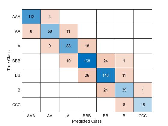
Find the classification accuracy of the model on the test data set. Visualize the results by using a confusion matrix.
testAccuracy = 1 - loss(Mdl,creditTest,"Rating", ...
    LossFun="classiferror")
testAccuracy =
0.8104
confusionchart(creditTest.Rating,predict(Mdl,creditTest))

The model has all predicted classes within one unit of the true classes, meaning all predictions are off by no more than one rating.
Input Arguments
Name-Value Arguments
Output Arguments
More About
The default neural network classifier has the following layer structure.
| Structure | Description |
|---|---|
|
| Input — This layer corresponds to the predictor data in
Tbl or X. |
First fully connected layer — This layer has 10 outputs by default.
| |
ReLU activation function —
| |
Final fully connected layer — This layer has K outputs, where K is the number of classes in the response variable.
| |
Softmax function (for both binary and multiclass classification) —
The results correspond to the predicted classification scores (or posterior probabilities). | |
| Output — This layer corresponds to the predicted class labels. |
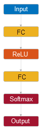
For an example that shows how a neural network classifier with this layer structure returns predictions, see Predict Using Layer Structure of Neural Network Classifier.
To specify a custom neural network architecture, use the
Network
argument. (since R2025a)
Tips
Always try to standardize the numeric predictors (see
Standardize). Standardization makes predictors insensitive to the scales on which they are measured.After training a model, you can generate C/C++ code that predicts labels for new data. Generating C/C++ code requires MATLAB Coder™. For details, see Introduction to Code Generation for Statistics and Machine Learning Functions.
To build deeper networks, you can use the
dlnetwork(Deep Learning Toolbox) function to convert your network to adlnetworkobject (since R2024b), or you can open your network in the Deep Network Designer (Deep Learning Toolbox) app (since R2026a). Usedlnetworkobjects to make further edits and customize the underlying neural network.
Algorithms
References
[1] Glorot, Xavier, and Yoshua Bengio. “Understanding the difficulty of training deep feedforward neural networks.” In Proceedings of the thirteenth international conference on artificial intelligence and statistics, pp. 249–256. 2010.
[2] He, Kaiming, Xiangyu Zhang, Shaoqing Ren, and Jian Sun. “Delving deep into rectifiers: Surpassing human-level performance on imagenet classification.” In Proceedings of the IEEE international conference on computer vision, pp. 1026–1034. 2015.
[3] Nocedal, J. and S. J. Wright. Numerical Optimization, 2nd ed., New York: Springer, 2006.
Extended Capabilities
Version History
Introduced in R2021aSee Also
ClassificationNeuralNetwork | predict | loss | hyperparameters | margin | edge | ClassificationPartitionedNeuralNetwork | CompactClassificationNeuralNetwork | countPredictorsAfterCategoricalEncoding | dlnetwork (Deep Learning Toolbox)