fitcgam
Syntax
Description
Mdl = fitcgam(Tbl,ResponseVarName)Mdl trained using the sample data contained in the table
            Tbl. The input argument ResponseVarName is the
          name of the variable in Tbl that contains the class labels for binary
          classification.
Mdl = fitcgam(___,Name,Value)'Interactions',5 specifies to include five interaction terms in the
          model. You can also specify a list of interaction terms using the
            Interactions name-value argument.
[
          also returns Mdl,AggregateOptimizationResults] = fitcgam(___)AggregateOptimizationResults, which contains
          hyperparameter optimization results when you specify the
            OptimizeHyperparameters and
            HyperparameterOptimizationOptions name-value arguments. You must
          also specify the ConstraintType and
            ConstraintBounds options of
            HyperparameterOptimizationOptions. You can use this syntax to
          optimize on compact model size instead of cross-validation loss, and to perform a set of
          multiple optimization problems that have the same options but different constraint
          bounds.
Examples
Train a univariate generalized additive model, which contains linear terms for predictors. Then, interpret the prediction for a specified data instance by using the plotLocalEffects function.
Load the ionosphere data set. This data set has 34 predictors and 351 binary responses for radar returns, either bad ('b') or good ('g').
load ionosphereTrain a univariate GAM that identifies whether the radar return is bad ('b') or good ('g'). 
Mdl = fitcgam(X,Y)
Mdl = 
  ClassificationGAM
             ResponseName: 'Y'
    CategoricalPredictors: []
               ClassNames: {'b'  'g'}
           ScoreTransform: 'logit'
                Intercept: 2.2715
          NumObservations: 351
  Properties, Methods
Mdl is a ClassificationGAM model object. The model display shows a partial list of the model properties. To view the full list of properties, double-click the variable name Mdl in the Workspace. The Variables editor opens for Mdl. Alternatively, you can display the properties in the Command Window by using dot notation. For example, display the class order of Mdl.
classOrder = Mdl.ClassNames
classOrder = 2×1 cell
    {'b'}
    {'g'}
Classify the first observation of the training data, and plot the local effects of the terms in Mdl on the prediction.
label = predict(Mdl,X(1,:))
label = 1×1 cell array
    {'g'}
plotLocalEffects(Mdl,X(1,:))

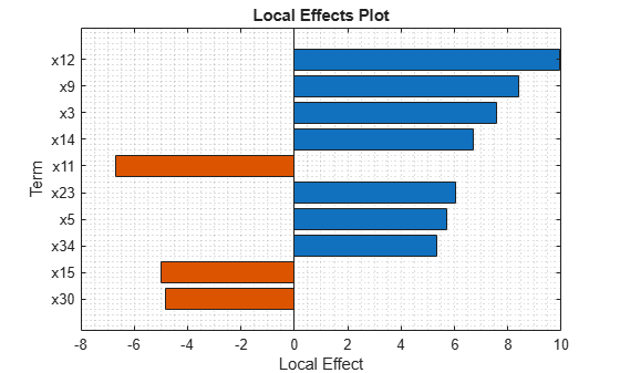
The predict function classifies the first observation X(1,:) as 'g'. The plotLocalEffects function creates a horizontal bar graph that shows the local effects of the 10 most important terms on the prediction. Each local effect value shows the contribution of each term to the classification score for 'g', which is the logit of the posterior probability that the classification is 'g' for the observation.
Train a generalized additive model that contains linear and interaction terms for predictors in three different ways:
- Specify the interaction terms using the - formulainput argument.
- Specify the - 'Interactions'name-value argument.
- Build a model with linear terms first and add interaction terms to the model by using the - addInteractionsfunction.
Load Fisher's iris data set. Create a table that contains observations for versicolor and virginica.
load fisheriris inds = strcmp(species,'versicolor') | strcmp(species,'virginica'); tbl = array2table(meas(inds,:),'VariableNames',["x1","x2","x3","x4"]); tbl.Y = species(inds,:);
Specify formula
Train a GAM that contains the four linear terms (x1, x2, x3, and x4) and two interaction terms (x1*x2 and x2*x3). Specify the terms using a formula in the form 'Y ~ terms'.
Mdl1 = fitcgam(tbl,'Y ~ x1 + x2 + x3 + x4 + x1:x2 + x2:x3');The function adds interaction terms to the model in the order of importance. You can use the Interactions property to check the interaction terms in the model and the order in which fitcgam adds them to the model. Display the Interactions property.
Mdl1.Interactions
ans = 2×2
     2     3
     1     2
Each row of Interactions represents one interaction term and contains the column indexes of the predictor variables for the interaction term.
Specify 'Interactions'
Pass the training data (tbl) and the name of the response variable in tbl to fitcgam, so that the function includes the linear terms for all the other variables as predictors. Specify the 'Interactions' name-value argument using a logical matrix to include the two interaction terms, x1*x2 and x2*x3. 
Mdl2 = fitcgam(tbl,'Y','Interactions',logical([1 1 0 0; 0 1 1 0])); Mdl2.Interactions
ans = 2×2
     2     3
     1     2
You can also specify 'Interactions' as the number of interaction terms or as 'all' to include all available interaction terms. Among the specified interaction terms, fitcgam identifies those whose p-values are not greater than the 'MaxPValue' value and adds them to the model. The default 'MaxPValue' is 1 so that the function adds all specified interaction terms to the model.
Specify 'Interactions','all' and set the 'MaxPValue' name-value argument to 0.01.
Mdl3 = fitcgam(tbl,'Y','Interactions','all','MaxPValue',0.01); Mdl3.Interactions
ans = 5×2
     3     4
     2     4
     1     4
     2     3
     1     3
Mdl3 includes five of the six available pairs of interaction terms. 
Use addInteractions Function
Train a univariate GAM that contains linear terms for predictors, and then add interaction terms to the trained model by using the addInteractions function. Specify the second input argument of addInteractions in the same way you specify the 'Interactions' name-value argument of fitcgam. You can specify the list of interaction terms using a logical matrix, the number of interaction terms, or 'all'. 
Specify the number of interaction terms as 5 to add the five most important interaction terms to the trained model.
Mdl4 = fitcgam(tbl,'Y');
UpdatedMdl4 = addInteractions(Mdl4,5);
UpdatedMdl4.Interactionsans = 5×2
     3     4
     2     4
     1     4
     2     3
     1     3
Mdl4 is a univariate GAM, and UpdatedMdl4 is an updated GAM that contains all the terms in Mdl4 and five additional interaction terms.
Train a cross-validated GAM with 10 folds, which is the default cross-validation option, by using fitcgam. Then, use kfoldPredict to predict class labels for validation-fold observations using a model trained on training-fold observations.
Load the ionosphere data set. This data set has 34 predictors and 351 binary responses for radar returns, either bad ('b') or good ('g').
load ionosphereCreate a cross-validated GAM by using the default cross-validation option. Specify the 'CrossVal' name-value argument as 'on'. 
rng('default') % For reproducibility CVMdl = fitcgam(X,Y,'CrossVal','on')
CVMdl = 
  ClassificationPartitionedGAM
    CrossValidatedModel: 'GAM'
         PredictorNames: {'x1'  'x2'  'x3'  'x4'  'x5'  'x6'  'x7'  'x8'  'x9'  'x10'  'x11'  'x12'  'x13'  'x14'  'x15'  'x16'  'x17'  'x18'  'x19'  'x20'  'x21'  'x22'  'x23'  'x24'  'x25'  'x26'  'x27'  'x28'  'x29'  'x30'  'x31'  'x32'  'x33'  'x34'}
           ResponseName: 'Y'
        NumObservations: 351
                  KFold: 10
              Partition: [1×1 cvpartition]
      NumTrainedPerFold: [1×1 struct]
             ClassNames: {'b'  'g'}
         ScoreTransform: 'logit'
  Properties, Methods
The fitcgam function creates a ClassificationPartitionedGAM model object CVMdl with 10 folds. During cross-validation, the software completes these steps:
- Randomly partition the data into 10 sets. 
- For each set, reserve the set as validation data, and train the model using the other 9 sets. 
- Store the 10 compact, trained models in a 10-by-1 cell vector in the - Trainedproperty of the cross-validated model object- ClassificationPartitionedGAM.
You can override the default cross-validation setting by using the 'CVPartition', 'Holdout', 'KFold', or 'Leaveout' name-value argument. 
Classify the observations in X by using kfoldPredict. The function predicts class labels for every observation using the model trained without that observation.
label = kfoldPredict(CVMdl);
Create a confusion matrix to compare the true classes of the observations to their predicted labels.
C = confusionchart(Y,label);

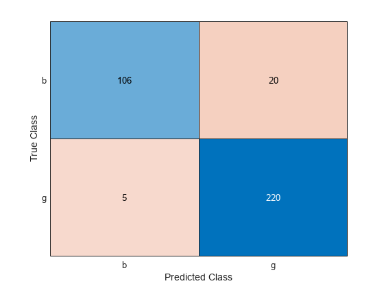
Compute the classification error.
L = kfoldLoss(CVMdl)
L = 0.0712
The average misclassification rate over 10 folds is about 7%.
Optimize the hyperparameters of a GAM with respect to cross-validation loss by using the OptimizeHyperparameters name-value argument.
Load the 1994 census data stored in census1994.mat. The data set consists of demographic data from the US Census Bureau to predict whether an individual makes over $50,000 per year. The classification task is to fit a model that predicts the salary category of people given their age, working class, education level, marital status, race, and so on.
load census1994census1994 contains the training data set adultdata and the test data set adulttest. To reduce the running time for this example, subsample 500 training observations and 500 test observations by using the datasample function. 
rng('default') NumSamples = 5e2; adultdata = datasample(adultdata,NumSamples,'Replace',false); adulttest = datasample(adulttest,NumSamples,'Replace',false);
Train a GAM classifier by passing the training data adultdata to the fitcgam function, and include the OptimizeHyperparameters argument. Specify OptimizeHyperparameters as 'auto' so that fitcgam finds optimal values of InitialLearnRateForPredictors, NumTreesPerPredictor, Interactions, InitialLearnRateForInteractions, and NumTreesPerInteraction. For reproducibility, choose the 'expected-improvement-plus' acquisition function. The default acquisition function depends on run time and, therefore, can give varying results.
Mdl = fitcgam(adultdata,'salary','OptimizeHyperparameters','auto', ... 'HyperparameterOptimizationOptions', ... struct('AcquisitionFunctionName','expected-improvement-plus'))
|==========================================================================================================================================================| | Iter | Eval | Objective | Objective | BestSoFar | BestSoFar | InitialLearnRate-| NumTreesPerP-| Interactions | InitialLearnRate-| NumTreesPerI-| | | result | | runtime | (observed) | (estim.) | ForPredictors | redictor | | ForInteractions | nteraction | |==========================================================================================================================================================| | 1 | Best | 0.148 | 11.721 | 0.148 | 0.148 | 0.001555 | 356 | 5 | 0.068117 | 16 | | 2 | Accept | 0.182 | 0.88258 | 0.148 | 0.14977 | 0.94993 | 25 | 0 | - | - | | 3 | Accept | 0.174 | 0.5938 | 0.148 | 0.148 | 0.016784 | 11 | 3 | 0.12025 | 12 | | 4 | Accept | 0.176 | 10.466 | 0.148 | 0.148 | 0.14207 | 179 | 71 | 0.0020629 | 22 | | 5 | Accept | 0.176 | 9.6859 | 0.148 | 0.1502 | 0.0010025 | 104 | 12 | 0.0052651 | 178 | | 6 | Accept | 0.152 | 9.212 | 0.148 | 0.15035 | 0.0017566 | 323 | 4 | 0.079281 | 16 | | 7 | Accept | 0.166 | 16.319 | 0.148 | 0.14801 | 0.0011656 | 497 | 10 | 0.17479 | 92 | | 8 | Accept | 0.172 | 10.99 | 0.148 | 0.14914 | 0.0014435 | 397 | 0 | - | - | | 9 | Accept | 0.16 | 11.9 | 0.148 | 0.14801 | 0.0016398 | 432 | 2 | 0.045129 | 11 | | 10 | Accept | 0.172 | 4.414 | 0.148 | 0.14855 | 0.0013589 | 146 | 9 | 0.065204 | 12 | | 11 | Accept | 0.156 | 10.724 | 0.148 | 0.14911 | 0.002082 | 368 | 7 | 0.0011513 | 12 | | 12 | Accept | 0.178 | 11.031 | 0.148 | 0.14801 | 0.13309 | 360 | 6 | 0.67104 | 13 | | 13 | Accept | 0.154 | 11.475 | 0.148 | 0.15192 | 0.0014287 | 380 | 5 | 0.027919 | 18 | | 14 | Accept | 0.164 | 10.497 | 0.148 | 0.15151 | 0.0015368 | 318 | 5 | 0.022401 | 93 | | 15 | Best | 0.144 | 9.6966 | 0.144 | 0.14515 | 0.0020403 | 331 | 8 | 0.12167 | 11 | | 16 | Accept | 0.168 | 9.6039 | 0.144 | 0.14401 | 0.0016201 | 329 | 10 | 0.74319 | 12 | | 17 | Accept | 0.16 | 9.0822 | 0.144 | 0.1526 | 0.002317 | 313 | 9 | 0.093554 | 18 | | 18 | Accept | 0.158 | 9.8266 | 0.144 | 0.15425 | 0.0016865 | 331 | 5 | 0.023535 | 11 | | 19 | Accept | 0.146 | 11.464 | 0.144 | 0.15096 | 0.0019238 | 386 | 6 | 0.043578 | 14 | | 20 | Accept | 0.156 | 11.165 | 0.144 | 0.15234 | 0.0023502 | 385 | 6 | 0.063029 | 11 | |==========================================================================================================================================================| | Iter | Eval | Objective | Objective | BestSoFar | BestSoFar | InitialLearnRate-| NumTreesPerP-| Interactions | InitialLearnRate-| NumTreesPerI-| | | result | | runtime | (observed) | (estim.) | ForPredictors | redictor | | ForInteractions | nteraction | |==========================================================================================================================================================| | 21 | Accept | 0.146 | 11.203 | 0.144 | 0.15105 | 0.0023381 | 383 | 6 | 0.042149 | 21 | | 22 | Best | 0.142 | 11.922 | 0.142 | 0.14959 | 0.0024173 | 400 | 7 | 0.022884 | 18 | | 23 | Accept | 0.152 | 13.325 | 0.142 | 0.14972 | 0.0017718 | 443 | 8 | 0.022974 | 18 | | 24 | Best | 0.14 | 12.785 | 0.14 | 0.14681 | 0.0032302 | 417 | 7 | 0.01295 | 23 | | 25 | Accept | 0.148 | 11.121 | 0.14 | 0.14672 | 0.0043102 | 371 | 6 | 0.016624 | 27 | | 26 | Accept | 0.14 | 11.871 | 0.14 | 0.14433 | 0.0029528 | 410 | 6 | 0.011766 | 25 | | 27 | Accept | 0.15 | 13.058 | 0.14 | 0.14441 | 0.0038288 | 455 | 6 | 0.038686 | 14 | | 28 | Accept | 0.144 | 13.992 | 0.14 | 0.14374 | 0.0030969 | 471 | 7 | 0.0093565 | 39 | | 29 | Accept | 0.144 | 14.149 | 0.14 | 0.14331 | 0.0033063 | 487 | 5 | 0.0033831 | 26 | | 30 | Best | 0.138 | 12.442 | 0.138 | 0.14213 | 0.0031221 | 420 | 5 | 0.0035267 | 26 |

__________________________________________________________
Optimization completed.
MaxObjectiveEvaluations of 30 reached.
Total function evaluations: 30
Total elapsed time: 326.2596 seconds
Total objective function evaluation time: 316.6185
Best observed feasible point:
    InitialLearnRateForPredictors    NumTreesPerPredictor    Interactions    InitialLearnRateForInteractions    NumTreesPerInteraction
    _____________________________    ____________________    ____________    _______________________________    ______________________
              0.0031221                      420                  5                     0.0035267                         26          
Observed objective function value = 0.138
Estimated objective function value = 0.14267
Function evaluation time = 12.4417
Best estimated feasible point (according to models):
    InitialLearnRateForPredictors    NumTreesPerPredictor    Interactions    InitialLearnRateForInteractions    NumTreesPerInteraction
    _____________________________    ____________________    ____________    _______________________________    ______________________
              0.0029528                      410                  6                     0.011766                          25          
Estimated objective function value = 0.14213
Estimated function evaluation time = 12.2594
Mdl = 
  ClassificationGAM
                       PredictorNames: {'age'  'workClass'  'fnlwgt'  'education'  'education_num'  'marital_status'  'occupation'  'relationship'  'race'  'sex'  'capital_gain'  'capital_loss'  'hours_per_week'  'native_country'}
                         ResponseName: 'salary'
                CategoricalPredictors: [2 4 6 7 8 9 10 14]
                           ClassNames: [<=50K    >50K]
                       ScoreTransform: 'logit'
                            Intercept: -1.3924
                         Interactions: [6×2 double]
                      NumObservations: 500
    HyperparameterOptimizationResults: [1×1 BayesianOptimization]
  Properties, Methods
fitcgam returns a ClassificationGAM model object that uses the best estimated feasible point. The best estimated feasible point is the set of hyperparameters that minimizes the upper confidence bound of the cross-validation loss based on the underlying Gaussian process model of the Bayesian optimization process. 
The Bayesian optimization process internally maintains a Gaussian process model of the objective function. The objective function is the cross-validated misclassification rate for classification. For each iteration, the optimization process updates the Gaussian process model and uses the model to find a new set of hyperparameters. Each line of the iterative display shows the new set of hyperparameters and these column values:
- Objective— Objective function value computed at the new set of hyperparameters.
- Objective runtime— Objective function evaluation time.
- Eval result— Result report, specified as- Accept,- Best, or- Error.- Acceptindicates that the objective function returns a finite value, and- Errorindicates that the objective function returns a value that is not a finite real scalar.- Bestindicates that the objective function returns a finite value that is lower than previously computed objective function values.
- BestSoFar(observed)— The minimum objective function value computed so far. This value is either the objective function value of the current iteration (if the- Eval resultvalue for the current iteration is- Best) or the value of the previous- Bestiteration.
- BestSoFar(estim.)— At each iteration, the software estimates the upper confidence bounds of the objective function values, using the updated Gaussian process model, at all the sets of hyperparameters tried so far. Then the software chooses the point with the minimum upper confidence bound. The- BestSoFar(estim.)value is the objective function value returned by the- predictObjectivefunction at the minimum point.
The plot below the iterative display shows the BestSoFar(observed) and BestSoFar(estim.) values in blue and green, respectively.
The returned object Mdl uses the best estimated feasible point, that is, the set of hyperparameters that produces the BestSoFar(estim.) value in the final iteration based on the final Gaussian process model. 
Obtain the best estimated feasible point from Mdl in the HyperparameterOptimizationResults property.
Mdl.HyperparameterOptimizationResults.XAtMinEstimatedObjective
ans=1×5 table
    InitialLearnRateForPredictors    NumTreesPerPredictor    Interactions    InitialLearnRateForInteractions    NumTreesPerInteraction
    _____________________________    ____________________    ____________    _______________________________    ______________________
              0.0029528                      410                  6                     0.011766                          25          
Alternatively, you can use the bestPoint function. By default, the bestPoint function uses the 'min-visited-upper-confidence-interval' criterion.
[x,CriterionValue,iteration] = bestPoint(Mdl.HyperparameterOptimizationResults)
x=1×5 table
    InitialLearnRateForPredictors    NumTreesPerPredictor    Interactions    InitialLearnRateForInteractions    NumTreesPerInteraction
    _____________________________    ____________________    ____________    _______________________________    ______________________
              0.0029528                      410                  6                     0.011766                          25          
CriterionValue = 0.1464
iteration = 26
The 'min-visited-upper-confidence-interval' criterion chooses the hyperparameters obtained from the 26th iteration as the best point. CriterionValue is the upper bound of the cross-validated loss computed by the final Gaussian process model.
You can also extract the best observed feasible point (that is, the last Best point in the iterative display) from the HyperparameterOptimizationResults property or by specifying Criterion as 'min-observed'.
Mdl.HyperparameterOptimizationResults.XAtMinObjective
ans=1×5 table
    InitialLearnRateForPredictors    NumTreesPerPredictor    Interactions    InitialLearnRateForInteractions    NumTreesPerInteraction
    _____________________________    ____________________    ____________    _______________________________    ______________________
              0.0031221                      420                  5                     0.0035267                         26          
[x_observed,CriterionValue_observed,iteration_observed] = bestPoint(Mdl.HyperparameterOptimizationResults,'Criterion','min-observed')
x_observed=1×5 table
    InitialLearnRateForPredictors    NumTreesPerPredictor    Interactions    InitialLearnRateForInteractions    NumTreesPerInteraction
    _____________________________    ____________________    ____________    _______________________________    ______________________
              0.0031221                      420                  5                     0.0035267                         26          
CriterionValue_observed = 0.1380
iteration_observed = 30
The 'min-observed' criterion chooses the hyperparameters obtained from the 30th iteration as the best point. CriterionValue_observed is the actual cross-validated loss computed using the selected hyperparameters. For more information, see the Criterion name-value argument of bestPoint.
Evaluate the performance of the classifier on the test set by computing the test set classification error.
L = loss(Mdl,adulttest,'salary')L = 0.1564
Optimize the parameters of a GAM with respect to cross-validation by using the bayesopt function.
Alternatively, you can find optimal values of fitcgam name-value arguments by using the OptimizeHyperparameters name-value argument. For an example, see Optimize GAM Using OptimizeHyperparameters.
Load the 1994 census data stored in census1994.mat. The data set consists of demographic data from the US Census Bureau to predict whether an individual makes over $50,000 per year. The classification task is to fit a model that predicts the salary category of people given their age, working class, education level, marital status, race, and so on.
load census1994census1994 contains the training data set adultdata and the test data set adulttest. To reduce the running time for this example, subsample 500 training observations from adultdata by using the datasample function. 
rng('default') NumSamples = 5e2; adultdata = datasample(adultdata,NumSamples,'Replace',false);
Set up a partition for cross-validation. This step fixes the cross-validation sets that the optimization uses at each step.
c = cvpartition(adultdata.salary,'KFold',5);Prepare optimizableVariable objects for the name-value arguments that you want to optimize using Bayesian optimization. This example finds optimal values for the MaxNumSplitsPerPredictor and NumTreesPerPredictor arguments of fitcgam.
maxNumSplits = optimizableVariable('maxNumSplits',[1,10],'Type','integer'); numTrees = optimizableVariable('numTrees',[1,500],'Type','integer');
Create an objective function that takes an input z = [maxNumSplits,numTrees] and returns the cross-validated loss value of z.
minfun = @(z)kfoldLoss(fitcgam(adultdata,'salary','CVPartition',c, ... 'MaxNumSplitsPerPredictor',z.maxNumSplits, ... 'NumTreesPerPredictor',z.numTrees));
If you specify a cross-validation option, then the fitcgam function returns a cross-validated model object ClassificationPartitionedGAM. The kfoldLoss function returns the classification loss obtained by the cross-validated model. Therefore, the function handle minfun computes the cross-validation loss at the parameters in z.
Search for the best parameters [maxNumSplits,numTrees] using bayesopt. For reproducibility, choose the 'expected-improvement-plus' acquisition function. The default acquisition function depends on run time and, therefore, can give varying results. 
results = bayesopt(minfun,[maxNumSplits,numTrees],'Verbose',0, ... 'IsObjectiveDeterministic',true, ... 'AcquisitionFunctionName','expected-improvement-plus');


Obtain the best point from results.
zbest = bestPoint(results)
zbest=1×2 table
    maxNumSplits    numTrees
    ____________    ________
         1             5    
Train an optimized GAM using the zbest values.
Mdl = fitcgam(adultdata,'salary', ... 'MaxNumSplitsPerPredictor',zbest.maxNumSplits, ... 'NumTreesPerPredictor',zbest.numTrees);
Input Arguments
Sample data used to train the model, specified as a table. Each row of
              Tbl corresponds to one observation, and each column corresponds
            to one predictor variable. Multicolumn variables and cell arrays other than cell arrays
            of character vectors are not allowed.
Optionally, Tbl can contain a column for the response variable
            and a column for the observation weights.
- The response variable must be a categorical, character, or string array, a logical or numeric vector, or a cell array of character vectors. - fitcgamsupports only binary classification. Either the response variable must contain exactly two distinct classes, or you must specify two classes for training by using the- ClassNamesname-value argument.
- A good practice is to specify the order of the classes in the response variable by using the - ClassNamesname-value argument.
 
- The column for the weights must be a numeric vector. 
- You must specify the response variable in - Tblby using- ResponseVarNameor- formulaand specify the observation weights in- Tblby using- Weights.- Specify the response variable by using - ResponseVarName—- fitcgamuses the remaining variables as predictors. To use a subset of the remaining variables in- Tblas predictors, specify predictor variables by using- PredictorNames.
- Define a model specification by using - formula—- fitcgamuses a subset of the variables in- Tblas predictor variables and the response variable, as specified in- formula.
 
If Tbl does not contain the response variable, then specify a
            response variable by using Y. The length of the response variable
              Y and the number of rows in Tbl must be
            equal. To use a subset of the variables in Tbl as predictors,
            specify predictor variables by using PredictorNames.
fitcgam considers NaN,
              '' (empty character vector), "" (empty string),
              <missing>, and <undefined> values in
              Tbl to be missing values.
- fitcgamdoes not use observations with all missing values in the fit.
- fitcgamdoes not use observations with missing response values in the fit.
- fitcgamuses observations with some missing values for predictors to find splits on variables for which these observations have valid values.
Data Types: table
Response variable name, specified as a character vector or string scalar containing the name
            of the response variable in Tbl. For example, if the response
            variable Y is stored in Tbl.Y, then specify it as
                'Y'.
Data Types: char | string
Model specification, specified as a character vector or string scalar in the form
                'Y ~ terms'. The formula argument specifies
            a response variable and linear and interaction terms for predictor variables. Use
                formula to specify a subset of variables in
                Tbl as predictors for training the model. If you specify a
            formula, then the software does not use any variables in Tbl that
            do not appear in formula.
For example, specify 'Y~x1+x2+x3+x1:x2'. In this form,
                Y represents the response variable, and x1,
                x2, and x3 represent the linear terms for the
            predictor variables. x1:x2 represents the interaction term for
                x1 and x2.
The variable names in the formula must be both variable names in Tbl
            (Tbl.Properties.VariableNames) and valid MATLAB® identifiers. You can verify the variable names in Tbl by
        using the isvarname function. If the variable names
        are not valid, then you can convert them by using the matlab.lang.makeValidName function.
Alternatively, you can specify a response variable and linear terms for predictors
            using formula, and specify interaction terms for predictors using
                'Interactions'.
fitcgam builds a set of interaction trees using only the
            terms whose p-values are not greater than the
                'MaxPValue' value.
Example: 'Y~x1+x2+x3+x1:x2'
Data Types: char | string
Class labels, specified as a categorical, character, or string array, a logical or numeric vector, or a cell array of character vectors.
- fitcgamsupports only binary classification. Either- Ymust contain exactly two distinct classes, or you must specify two classes for training by using the- ClassNamesname-value argument.
- The length of - Ymust be equal to the number of observations in- Xor- Tbl.
- If - Yis a character array, then each label must correspond to one row of the array.
- A good practice is to specify the class order using the - ClassNamesname-value pair argument.
- fitcgamconsiders- NaN,- ''(empty character vector),- ""(empty string),- <missing>, and- <undefined>values in- Yto be missing values.- fitcgamdoes not use observations with missing response values in the fit.
Data Types: single | double | categorical | logical | char | string | cell
Predictor data, specified as a numeric matrix. Each row of X corresponds to one observation, and each column corresponds to one predictor variable.
fitcgam considers NaN values in
                X as missing values. The function does not use observations
            with all missing values in the fit. fitcgam uses observations
            with some missing values for X to find splits on variables for
            which these observations have valid values.
Data Types: single | double
Name-Value Arguments
Specify optional pairs of arguments as
      Name1=Value1,...,NameN=ValueN, where Name is
      the argument name and Value is the corresponding value.
      Name-value arguments must appear after other arguments, but the order of the
      pairs does not matter.
    
      Before R2021a, use commas to separate each name and value, and enclose 
      Name in quotes.
    
Example: 'Interactions','all','MaxPValue',0.05 specifies to include
        all available interaction terms whose p-values are not greater than
        0.05.
GAM Options
Initial learning rate of gradient boosting for interaction terms, specified as a numeric scalar in the interval (0,1].
For each boosting iteration for interaction trees,
                fitcgam starts fitting with the initial learning rate. The
              function halves the learning rate until it finds a rate that improves the model
              fit.
Training a model using a small learning rate requires more learning iterations, but often achieves better accuracy.
For more details about gradient boosting, see Gradient Boosting Algorithm.
Example: 'InitialLearnRateForInteractions',0.1
Data Types: single | double
Initial learning rate of gradient boosting for linear terms, specified as a numeric scalar in the interval (0,1].
For each boosting iteration for predictor trees, fitcgam
              starts fitting with the initial learning rate. The function halves the learning rate
              until it finds a rate that improves the model fit.
Training a model using a small learning rate requires more learning iterations, but often achieves better accuracy.
For more details about gradient boosting, see Gradient Boosting Algorithm.
Example: 'InitialLearnRateForPredictors',0.1
Data Types: single | double
Number or list of interaction terms to include in the candidate set S,
                specified as a nonnegative integer scalar, a logical matrix, or
                        'all'.
- Number of interaction terms, specified as a nonnegative integer — S includes the specified number of important interaction terms, selected based on the p-values of the terms. 
- List of interaction terms, specified as a logical matrix — S includes the terms specified by a - t-by-- plogical matrix, where- tis the number of interaction terms, and- pis the number of predictors used to train the model. For example,- logical([1 1 0; 0 1 1])represents two pairs of interaction terms: a pair of the first and second predictors, and a pair of the second and third predictors.- If - fitcgamuses a subset of input variables as predictors, then the function indexes the predictors using only the subset. That is, the column indexes of the logical matrix do not count the response and observation weight variables. The indexes also do not count any variables not used by the function.
- 'all'— S includes all possible pairs of interaction terms, which is- p*(p – 1)/2number of terms in total.
Among the interaction terms in S, the fitcgam
                function identifies those whose p-values are not greater than the
                        'MaxPValue' value and uses them to build a set of
                interaction trees. Use the default value ('MaxPValue',1) to
                build interaction trees using all terms in S.
Example: 'Interactions','all'
Data Types: single | double | logical | char | string
Maximum number of decision splits (or branch nodes) for each interaction tree (boosted tree for an interaction term), specified as a positive integer scalar.
Example: 'MaxNumSplitsPerInteraction',5
Data Types: single | double
Maximum number of decision splits (or branch nodes) for each predictor tree (boosted tree for
                                                  a linear term), specified as a positive integer
                                                  scalar. By default,
                                                  fitcgam uses a tree stump
                                                  for a predictor tree.
Example: 'MaxNumSplitsPerPredictor',5
Data Types: single | double
Maximum p-value for detecting interaction terms, specified as a numeric scalar in the interval [0,1].
fitcgam first finds the candidate set S of
            interaction terms from formula or
                'Interactions'. Then the function identifies the interaction
            terms whose p-values are not greater than the
                'MaxPValue' value and uses them to build a set of interaction
            trees.
The default value ('MaxPValue',1) builds interaction trees for all
            interaction terms in the candidate set S.
For more details about detecting interaction terms, see Interaction Term Detection.
Example: 'MaxPValue',0.05
Data Types: single | double
Number of bins for numeric predictors, specified as a positive integer scalar or
                [] (empty).
- If you specify the - 'NumBins'value as a positive integer scalar (- numBins), then- fitcgambins every numeric predictor into at most- numBinsequiprobable bins, and then grows trees on the bin indices instead of the original data.- The number of bins can be less than - numBinsif a predictor has fewer than- numBinsunique values.
- fitcgamdoes not bin categorical predictors.
 
- If the - 'NumBins'value is empty (- []), then- fitcgamdoes not bin any predictors.
When you use a large training data set, this binning option speeds up training but might cause
            a decrease in accuracy. You can first use the default value of
                'NumBins', and then change the value depending on the accuracy
            and training speed.
The trained model Mdl stores the bin edges in the
                BinEdges property.
Example: 'NumBins',50
Data Types: single | double
Number of trees per interaction term, specified as a positive integer scalar.
The 'NumTreesPerInteraction' value is equivalent to the number of
            gradient boosting iterations for the interaction terms for predictors. For each
            iteration, fitcgam adds a set of interaction trees to the
            model, one tree for each interaction term. To learn about the gradient boosting
            algorithm, see Gradient Boosting Algorithm.
You can determine whether the fitted model has the specified number of trees by
            viewing the diagnostic message displayed when 'Verbose' is 1 or 2,
            or by checking the ReasonForTermination property value of the model
                Mdl.
Example: 'NumTreesPerInteraction',500
Data Types: single | double
Number of trees per linear term, specified as a positive integer scalar.
The 'NumTreesPerPredictor' value is equivalent to the number of
            gradient boosting iterations for the linear terms for predictors. For each iteration,
                fitcgam adds a set of predictor trees to the model, one
            tree for each predictor. To learn about the gradient boosting algorithm, see Gradient Boosting Algorithm.
You can determine whether the fitted model has the specified number of trees by
            viewing the diagnostic message displayed when 'Verbose' is 1 or 2,
            or by checking the ReasonForTermination property value of the model
                Mdl.
Example: 'NumTreesPerPredictor',500
Data Types: single | double
Other Classification Options
Categorical predictors list, specified as one of the values in this table.
| Value | Description | 
|---|---|
| Vector of positive integers | Each entry in the vector is an index value indicating that the corresponding predictor is
        categorical. The index values are between 1 and  If  | 
| Logical vector | A  | 
| Character matrix | Each row of the matrix is the name of a predictor variable. The names must match the entries in PredictorNames. Pad the names with extra blanks so each row of the character matrix has the same length. | 
| String array or cell array of character vectors | Each element in the array is the name of a predictor variable. The names must match the entries in PredictorNames. | 
| "all" | All predictors are categorical. | 
By default, if the predictor data is a table
        (Tbl), fitcgam assumes that a variable is
    categorical if it is a logical vector, unordered categorical vector, character array, string
    array, or cell array of character vectors. If the predictor data is a matrix
        (X), fitcgam assumes that all predictors are
    continuous. To identify any other predictors as categorical predictors, specify them by using
    the CategoricalPredictors name-value argument.
Example: 'CategoricalPredictors','all'
Data Types: single | double | logical | char | string | cell
Names of classes to use for training, specified as a categorical, character, or string
            array; a logical or numeric vector; or a cell array of character vectors.
                ClassNames must have the same data type as the response variable
            in Tbl or Y.
If ClassNames is a character array, then each element must correspond to one row of the array.
Use ClassNames to:
- Specify the order of the classes during training. 
- Specify the order of any input or output argument dimension that corresponds to the class order. For example, use - ClassNamesto specify the order of the dimensions of- Costor the column order of classification scores returned by- predict.
- Select a subset of classes for training. For example, suppose that the set of all distinct class names in - Yis- ["a","b","c"]. To train the model using observations from classes- "a"and- "c"only, specify- ClassNames=["a","c"].
The default value for ClassNames is the set of all distinct class names in the response variable in Tbl or Y.
Example: ClassNames=["b","g"]
Data Types: categorical | char | string | logical | single | double | cell
Misclassification cost of a point, specified as one of the following:
- 2-by-2 numeric matrix, where - Cost(i,j)is the cost of classifying a point into class- jif its true class is- i(that is, the rows correspond to the true class and the columns correspond to the predicted class). To specify the class order for the corresponding rows and columns of- Cost, set the- 'ClassNames'name-value argument.
- Structure - Swith two fields:- S.ClassNames, which contains the group names as a variable of the same data type as the response variable in- Tblor- Y; and- S.ClassificationCosts, which contains the cost matrix.
Example: 'Cost',[0 2; 1 0]
Data Types: single | double | struct
Number of iterations between diagnostic message printouts, specified as a nonnegative integer
                scalar. This argument is valid only when you specify 'Verbose'
                as 1.
If you specify 'Verbose',1 and 'NumPrint',numPrint, then
                the software displays diagnostic messages every numPrint
                iterations in the Command Window.
Example: 'NumPrint',500
Data Types: single | double
Predictor variable names, specified as a string array of unique names or cell array of unique
            character vectors. The functionality of PredictorNames depends on the
            way you supply the training data.
- If you supply - Xand- Y, then you can use- PredictorNamesto assign names to the predictor variables in- X.- The order of the names in - PredictorNamesmust correspond to the column order of- X. That is,- PredictorNames{1}is the name of- X(:,1),- PredictorNames{2}is the name of- X(:,2), and so on. Also,- size(X,2)and- numel(PredictorNames)must be equal.
- By default, - PredictorNamesis- {'x1','x2',...}.
 
- If you supply - Tbl, then you can use- PredictorNamesto choose which predictor variables to use in training. That is,- fitcgamuses only the predictor variables in- PredictorNamesand the response variable during training.- PredictorNamesmust be a subset of- Tbl.Properties.VariableNamesand cannot include the name of the response variable.
- By default, - PredictorNamescontains the names of all predictor variables.
- A good practice is to specify the predictors for training using either - PredictorNamesor- formula, but not both.
 
Example: "PredictorNames",["SepalLength","SepalWidth","PetalLength","PetalWidth"]
Data Types: string | cell
Prior probabilities for each class, specified as one of the following:
- Character vector or string scalar. 
- Vector (one scalar value for each class). To specify the class order for the corresponding elements of - 'Prior', set the- 'ClassNames'name-value argument.
- Structure - Swith two fields.- S.ClassNamescontains the class names as a variable of the same type as the response variable in- Yor- Tbl.
- S.ClassProbscontains a vector of corresponding probabilities.
 
fitcgam normalizes the weights in each class
                ('Weights') to add up to the value of the prior probability of
            the respective class.
Example: 'Prior','uniform'
Data Types: char | string | single | double | struct
Response variable name, specified as a character vector or string scalar.
- If you supply - Y, then you can use- ResponseNameto specify a name for the response variable.
- If you supply - ResponseVarNameor- formula, then you cannot use- ResponseName.
Example: ResponseName="response"
Data Types: char | string
Score transformation, specified as a built-in transformation function name or function handle.
This table summarizes the available score transformations. Specify one using its corresponding character vector or string scalar.
| Value | Description | 
|---|---|
| "doublelogit" | 1/(1 + e–2x) | 
| "invlogit" | log(x / (1 – x)) | 
| "ismax" | Sets the score for the class with the largest score to 1, and sets the scores for all other classes to 0 | 
| "logit" | 1/(1 + e–x) | 
| "none"or"identity" | x (no transformation) | 
| "sign" | –1 for x < 0 0 for x = 0 1 for x > 0 | 
| "symmetric" | 2x – 1 | 
| "symmetricismax" | Sets the score for the class with the largest score to 1, and sets the scores for all other classes to –1 | 
| "symmetriclogit" | 2/(1 + e–x) – 1 | 
For a MATLAB function or a function you define, use its function handle for the score transform. The function handle must accept a matrix (the original scores) and return a matrix of the same size (the transformed scores).
This argument determines the output score computation for object functions such as
                predict,
                margin, and
                edge. Use
                'logit' (default) to compute posterior probabilities, and use
                'none' to compute the logit of posterior probabilities.
Example: 'ScoreTransform','none'
Data Types: char | string | function_handle
Verbosity level, specified as 0, 1, or
            2. The Verbose value controls the amount of
        information that the software displays in the Command Window.
This table summarizes the available verbosity level options.
| Value | Description | 
|---|---|
| 0 | The software displays no information. | 
| 1 | The software displays diagnostic messages every numPrintiterations, wherenumPrintis the'NumPrint'value. | 
| 2 | The software displays diagnostic messages at every iteration. | 
Each line of the diagnostic messages shows the information about each boosting iteration and includes the following columns:
- Type— Type of trained trees,- 1D(predictor trees, or boosted trees for linear terms for predictors) or- 2D(interaction trees, or boosted trees for interaction terms for predictors)
- NumTrees— Number of trees per linear term or interaction term that- fitcgamadded to the model so far
- Deviance— Deviance of the model
- RelTol— Relative change of model predictions: , where is a column vector of model predictions at iteration k
- LearnRate— Learning rate used for the current iteration
Example: 'Verbose',1
Data Types: single | double
Observation weights, specified as a vector of scalar values or the name of a
              variable in Tbl. The software weights the observations in each row
              of X or Tbl with the corresponding value in
                Weights. The size of Weights must equal the
              number of rows in X or Tbl.
If you specify the input data as a table Tbl, then
                Weights can be the name of a variable in Tbl
              that contains a numeric vector. In this case, you must specify
                Weights as a character vector or string scalar. For example, if
              the weights vector W is stored in Tbl.W, then
              specify it as 'W'.
fitcgam normalizes the weights in each class to add up to
              the value of the prior probability of the respective class. Inf weights are not supported.
Data Types: single | double | char | string
Note
You cannot use any cross-validation name-value argument together with the
            OptimizeHyperparameters name-value argument. You can modify the
        cross-validation for OptimizeHyperparameters only by using the
            HyperparameterOptimizationOptions name-value argument.
Cross-Validation Options
 Flag to train a cross-validated model, specified as 'on'
                        or 'off'.
If you specify 'on', then the software trains a
                        cross-validated model with 10 folds.
You can override this cross-validation setting using the
                                'CVPartition', 'Holdout',
                                'KFold', or 'Leaveout'
                        name-value argument. You can use only one cross-validation name-value
                        argument at a time to create a cross-validated model.
Alternatively, cross-validate after creating a model by passing
                                Mdl to crossval.
Example: 'Crossval','on'
Cross-validation partition, specified as a cvpartition object that specifies the type of cross-validation and the
            indexing for the training and validation sets.
To create a cross-validated model, you can specify only one of these four name-value
            arguments: CVPartition, Holdout,
                KFold, or Leaveout.
Example: Suppose you create a random partition for 5-fold cross-validation on 500
            observations by using cvp = cvpartition(500,KFold=5). Then, you can
            specify the cross-validation partition by setting
            CVPartition=cvp.
Fraction of the data used for holdout validation, specified as a scalar value in the range
            (0,1). If you specify Holdout=p, then the software completes these
            steps: 
- Randomly select and reserve - p*100% of the data as validation data, and train the model using the rest of the data.
- Store the compact trained model in the - Trainedproperty of the cross-validated model.
To create a cross-validated model, you can specify only one of these four name-value
            arguments: CVPartition, Holdout,
                KFold, or Leaveout.
Example: Holdout=0.1
Data Types: double | single
Number of folds to use in the cross-validated model, specified as a positive integer value
            greater than 1. If you specify KFold=k, then the software completes
            these steps:
- Randomly partition the data into - ksets.
- For each set, reserve the set as validation data, and train the model using the other - k– 1 sets.
- Store the - kcompact trained models in a- k-by-1 cell vector in the- Trainedproperty of the cross-validated model.
To create a cross-validated model, you can specify only one of these four name-value
            arguments: CVPartition, Holdout,
                KFold, or Leaveout.
Example: KFold=5
Data Types: single | double
Leave-one-out cross-validation flag, specified as "on" or
                "off". If you specify Leaveout="on", then for
            each of the n observations (where n is the number
            of observations, excluding missing observations, specified in the
                NumObservations property of the model), the software completes
            these steps: 
- Reserve the one observation as validation data, and train the model using the other n – 1 observations. 
- Store the n compact trained models in an n-by-1 cell vector in the - Trainedproperty of the cross-validated model.
To create a cross-validated model, you can specify only one of these four name-value
            arguments: CVPartition, Holdout,
                KFold, or Leaveout.
Example: Leaveout="on"
Data Types: char | string
Hyperparameter Optimization Options
Parameters to optimize, specified as one of these values:
- 'none'— Do not optimize.
- 'auto'— Optimize- InitialLearnRateForPredictors,- NumTreesPerPredictor,- Interactions,- InitialLearnRateForInteractions, and- NumTreesPerInteraction.
- 'auto-univariate'— Optimize- InitialLearnRateForPredictorsand- NumTreesPerPredictor.
- 'auto-bivariate'— Optimize- Interactions,- InitialLearnRateForInteractions, and- NumTreesPerInteraction.
- 'all'— Optimize all eligible parameters.
- 'all-univariate'— Optimize all eligible univariate parameters.
- 'all-bivariate'— Optimize all eligible bivariate parameters.
- String array or cell array of eligible parameter names. 
- Vector of - optimizableVariableobjects, typically the output of- hyperparameters.
The eligible parameters for fitcgam are:
- Univariate hyperparameters - InitialLearnRateForPredictors—- fitcgamsearches among real values, log-scaled in the range- [1e-3,1].
- MaxNumSplitsPerPredictor—- fitcgamsearches among integers in the range- [1,maxNumSplits], where- maxNumSplitsis- min(30,max(2,NumObservations–1)).- NumObservationsis the number of observations, excluding missing observations, stored in the- NumObservationsproperty of the returned model- Mdl.
- NumTreesPerPredictor—- fitcgamsearches among integers, log-scaled in the range- [10,500].
 
- Bivariate hyperparameters - Interactions—- fitcgamsearches among integers, log-scaled in the range- [0,MaxNumInteractions]t, where- MaxNumInteractionsis- NumPredictors*(NumPredictors – 1)/2, and- NumPredictorsis the number of predictors used to train the model.
- InitialLearnRateForInteractions—- fitcgamsearches among real values, log-scaled in the range- [1e-3,1].
- MaxNumSplitsPerInteraction—- fitcgamsearches among integers in the range- [1,maxNumSplits].
- NumTreesPerInteraction—- fitcgamsearches among integers, log-scaled in the range- [10,500].
 
Use 'auto' or 'all' to find optimal
              hyperparameter values for both univariate and bivariate parameters. Alternatively, you
              can find optimal values for univariate parameters using
                'auto-univariate' or 'all-univariate' and then
              find optimal values for bivariate parameters using 'auto-bivariate'
              or 'all-bivariate'. For examples, see Optimize GAM Using OptimizeHyperparameters and Train Generalized Additive Model for Binary Classification.
The optimization attempts to minimize the cross-validation loss
    (error) for fitcgam by varying the parameters. To control the
    cross-validation type and other aspects of the optimization, use the
        HyperparameterOptimizationOptions name-value argument. When you use
        HyperparameterOptimizationOptions, you can use the (compact) model size
    instead of the cross-validation loss as the optimization objective by setting the
        ConstraintType and ConstraintBounds options.
Note
The values of OptimizeHyperparameters override any values you
            specify using other name-value arguments. For example, setting
                OptimizeHyperparameters to "auto" causes
                fitcgam to optimize hyperparameters corresponding to the
                "auto" option and to ignore any specified values for the
            hyperparameters.
Set nondefault parameters by passing a vector of
                optimizableVariable objects that have nondefault values. For
              example:
load fisheriris params = hyperparameters('fitcgam',meas,species); params(1).Range = [1e-4,1e6];
Pass params as the value of
                OptimizeHyperparameters.
By default, the iterative display appears at the command line,
    and plots appear according to the number of hyperparameters in the optimization. For the
    optimization and plots, the objective function is the misclassification rate. To control the
    iterative display, set the Verbose option of the
        HyperparameterOptimizationOptions name-value argument. To control the
    plots, set the ShowPlots field of the
        HyperparameterOptimizationOptions name-value argument.
Example: 'OptimizeHyperparameters','auto'
Options for optimization, specified as a HyperparameterOptimizationOptions object or a structure. This argument
            modifies the effect of the OptimizeHyperparameters name-value
            argument. If you specify HyperparameterOptimizationOptions, you must
            also specify OptimizeHyperparameters. All the options are optional.
            However, you must set ConstraintBounds and
                ConstraintType to return
                AggregateOptimizationResults. The options that you can set in a
            structure are the same as those in the
                HyperparameterOptimizationOptions object.
| Option | Values | Default | 
|---|---|---|
| Optimizer | 
 | "bayesopt" | 
| ConstraintBounds | Constraint bounds for N optimization problems,
                        specified as an N-by-2 numeric matrix or
                             | [] | 
| ConstraintTarget | Constraint target for the optimization problems, specified as
                             | If you specify ConstraintBoundsandConstraintType, then the default value is"matlab". Otherwise, the default value is[]. | 
| ConstraintType | Constraint type for the optimization problems, specified as
                             | [] | 
| AcquisitionFunctionName | Type of acquisition function: 
 
 Acquisition functions whose names include
                             | "expected-improvement-per-second-plus" | 
| MaxObjectiveEvaluations | Maximum number of objective function evaluations. If you specify multiple
                    optimization problems using ConstraintBounds, the value ofMaxObjectiveEvaluationsapplies to each optimization
                    problem individually. | 30for"bayesopt"and"randomsearch", and the entire grid for"gridsearch" | 
| MaxTime | Time limit for the optimization, specified as a nonnegative real
                        scalar. The time limit is in seconds, as measured by  | Inf | 
| NumGridDivisions | For Optimizer="gridsearch", the number of values in each
                    dimension. The value can be a vector of positive integers giving the number of
                    values for each dimension, or a scalar that applies to all dimensions. The
                    software ignores this option for categorical variables. | 10 | 
| ShowPlots | Logical value indicating whether to show plots of the optimization progress.
                    If this option is true, the software plots the best observed
                    objective function value against the iteration number. If you use Bayesian
                    optimization (Optimizer="bayesopt"), the
                    software also plots the best estimated objective function value. The best
                    observed objective function values and best estimated objective function values
                    correspond to the values in theBestSoFar (observed)andBestSoFar (estim.)columns of the iterative display,
                    respectively. You can find these values in the propertiesObjectiveMinimumTraceandEstimatedObjectiveMinimumTraceofMdl.HyperparameterOptimizationResults. If the problem
                    includes one or two optimization parameters for Bayesian optimization, thenShowPlotsalso plots a model of the objective function
                    against the parameters. | true | 
| SaveIntermediateResults | Logical value indicating whether to save the optimization results. If this
                    option is true, the software overwrites a workspace variable
                    named"BayesoptResults"at each iteration. The variable is aBayesianOptimizationobject. If you
                    specify multiple optimization problems usingConstraintBounds, the workspace variable is anAggregateBayesianOptimizationobject named"AggregateBayesoptResults". | false | 
| Verbose | Display level at the command line: 
 
For details, see the  | 1 | 
| UseParallel | Logical value indicating whether to run the Bayesian optimization in parallel, which requires Parallel Computing Toolbox™. Due to the nonreproducibility of parallel timing, parallel Bayesian optimization does not necessarily yield reproducible results. For details, see Parallel Bayesian Optimization. | false | 
| Repartition | Logical value indicating whether to repartition the cross-validation at
                        every iteration. If this option is  A value of
                             | false | 
| Specify only one of the following three options. | ||
| CVPartition | cvpartitionobject created bycvpartition | KFold=5if you do not specify a
                    cross-validation option | 
| Holdout | Scalar in the range (0,1)representing the holdout
                    fraction | |
| KFold | Integer greater than 1 | |
Example: HyperparameterOptimizationOptions=struct(UseParallel=true)
Output Arguments
Trained generalized additive model, returned as one of the model objects in this table.
| Model Object | Cross-Validation Options to Train Model Object | Ways to Classify Observations Using Model Object | 
|---|---|---|
| ClassificationGAM | None | Use predictto classify new observations, and useresubPredictto classify training observations. | 
| ClassificationPartitionedGAM | Specify KFold,Holdout,Leaveout,CrossVal, orCVPartition | Use kfoldPredictto classify
                      observations thatfitcgamholds out during training.kfoldPredictpredicts a class label for every
                      observation by using the model trained without that observation. | 
To reference properties of Mdl, use dot notation. For example,
            enter Mdl.Interactions in the Command Window to display the
            interaction terms in Mdl.
If you specify OptimizeHyperparameters and
    set the ConstraintType and ConstraintBounds options of
        HyperparameterOptimizationOptions, then Mdl is an
        N-by-1 cell array of model objects, where N is equal
    to the number of rows in ConstraintBounds. If none of the optimization
    problems yields a feasible model, then each cell array value is [].
Aggregate optimization results for multiple optimization problems, returned as an AggregateBayesianOptimization object. To return
                AggregateOptimizationResults, you must specify
                OptimizeHyperparameters and
                HyperparameterOptimizationOptions. You must also specify the
                ConstraintType and ConstraintBounds
            options of HyperparameterOptimizationOptions. For an example that
            shows how to produce this output, see Hyperparameter Optimization with Multiple Constraint Bounds.
More About
A generalized additive model (GAM) is an interpretable model that explains class scores (the logit of class probabilities) using a sum of univariate and bivariate shape functions of predictors.
fitcgam uses a boosted tree as a shape function for each predictor
        and, optionally, each pair of predictors; therefore, the function can capture a nonlinear
        relation between a predictor and the response variable. Because contributions of individual
        shape functions to the prediction (classification score) are well separated, the model is
        easy to interpret.
The standard GAM uses a univariate shape function for each predictor.
where y is a response variable that follows the binomial distribution with the probability of success (probability of positive class) μ in n observations. g(μ) is a logit link function, and c is an intercept (constant) term. fi(xi) is a univariate shape function for the ith predictor, which is a boosted tree for a linear term for the predictor (predictor tree).
You can include interactions between predictors in a model by adding bivariate shape functions of important interaction terms to the model.
where fij(xixj) is a bivariate shape function for the ith and jth predictors, which is a boosted tree for an interaction term for the predictors (interaction tree).
fitcgam finds important interaction terms based on the
            p-values of F-tests. For details, see Interaction Term Detection.
Deviance is a generalization of the residual sum of squares. It measures the goodness of fit compared to the saturated model.
The deviance of a fitted model is twice the difference between the loglikelihoods of the model and the saturated model:
-2(logL - logLs),
where L and Ls are the likelihoods of the fitted model and the saturated model, respectively. The saturated model is the model with the maximum number of parameters that you can estimate.
fitcgam uses the deviance to measure the goodness of model fit
        and finds a learning rate that reduces the deviance at each iteration. Specify
            'Verbose' as 1 or 2 to display the deviance and learning rate in
        the Command Window.
Algorithms
fitcgam fits a generalized additive model using a gradient
        boosting algorithm (Adaptive Logistic Regression).
fitcgam first builds sets of predictor trees (boosted trees for
        linear terms for predictors) and then builds sets of interaction trees (boosted trees for
        interaction terms for predictors). The boosting algorithm iterates for at most
          'NumTreesPerPredictor' times for predictor trees, and then iterates
        for at most 'NumTreesPerInteraction' times for interaction
        trees.
For each boosting iteration, fitcgam builds a set of predictor
        trees with the initial learning rate 'InitialLearnRateForPredictors',
        or builds a set of interaction trees with the initial learning rate
          'InitialLearnRateForInteractions'. 
- When building a set of trees, the function trains one tree at a time. It fits a tree to the residual that is the difference between the response and the aggregated prediction from all trees grown previously. To control the boosting learning speed, the function shrinks the tree by the learning rate and then adds the tree to the model and updates the residual. - Updated model = current model + (learning rate)·(new tree) 
- Updated residual = current residual – (learning rate)·(response explained by new tree) 
 
- If adding the set of trees improves the model fit (that is, reduces the deviance of the fit by a value larger than a tolerance), then - fitcgammoves to the next iteration.
- Otherwise, - fitcgamhalves the learning rate and uses it to update the model and residual. The function continues to halve the learning rate until it finds a rate that improves the model fit.- If the function cannot find such a learning rate when training predictor trees, then it stops boosting iterations for linear terms and starts boosting iterations for interaction terms. 
- If the function cannot find such a learning rate when training interaction trees, then it terminates the model fitting. 
 - You can determine why training stopped by checking the - ReasonForTerminationproperty of the trained model.
For each pairwise interaction term
                xixj
        (specified by formula or 'Interactions'), the
        software performs an F-test to examine whether the term is statistically
        significant.
To speed up the process, fitcgam bins numeric predictors into at
        most 8 equiprobable bins. The number of bins can be less than 8 if a predictor has fewer
        than 8 unique values. The F-test examines the null hypothesis that the
        bins created by xi and
                xj have equal responses versus the
        alternative that at least one bin has a different response value from the others. A small
            p-value indicates that differences are significant, which implies
        that the corresponding interaction term is significant and, therefore, including the term
        can improve the model fit.
fitcgam builds a set of interaction trees using the terms whose
            p-values are not greater than the 'MaxPValue'
        value. You can use the default 'MaxPValue' value 1
        to build interaction trees using all terms specified by formula or
            'Interactions'.
fitcgam adds interaction terms to the model in the order of
        importance based on the p-values. Use the
            Interactions property of the returned model to check the order of
        the interaction terms added to the model.
- If you specify the - Cost,- Prior, and- Weightsname-value arguments, the output model object stores the specified values in the- Cost,- Prior, and- Wproperties, respectively. The- Costproperty stores the user-specified cost matrix as is. The- Priorand- Wproperties store the prior probabilities and observation weights, respectively, after normalization. For details, see Misclassification Cost Matrix, Prior Probabilities, and Observation Weights.
- The software uses the - Costproperty for prediction, but not training. Therefore,- Costis not read-only; you can change the property value by using dot notation after creating the trained model.
References
[1] Lou, Yin, Rich Caruana, and Johannes Gehrke. "Intelligible Models for Classification and Regression." Proceedings of the 18th ACM SIGKDD International Conference on Knowledge Discovery and Data Mining (KDD ’12). Beijing, China: ACM Press, 2012, pp. 150–158.
[2] Lou, Yin, Rich Caruana, Johannes Gehrke, and Giles Hooker. "Accurate Intelligible Models with Pairwise Interactions." Proceedings of the 19th ACM SIGKDD International Conference on Knowledge Discovery and Data Mining (KDD ’13) Chicago, Illinois, USA: ACM Press, 2013, pp. 623–631.
Extended Capabilities
To perform parallel hyperparameter optimization, use the UseParallel=true
        option in the HyperparameterOptimizationOptions name-value argument in
        the call to the fitcgam function.
For more information on parallel hyperparameter optimization, see Parallel Bayesian Optimization.
For general information about parallel computing, see Run MATLAB Functions with Automatic Parallel Support (Parallel Computing Toolbox).
Version History
Introduced in R2021afitcgam defaults to serial hyperparameter optimization when
            HyperparameterOptimizationOptions includes
            UseParallel=true and the software cannot open a parallel pool.
In previous releases, the software issues an error under these circumstances.
MATLAB Command
You clicked a link that corresponds to this MATLAB command:
Run the command by entering it in the MATLAB Command Window. Web browsers do not support MATLAB commands.
Select a Web Site
Choose a web site to get translated content where available and see local events and offers. Based on your location, we recommend that you select: .
You can also select a web site from the following list
How to Get Best Site Performance
Select the China site (in Chinese or English) for best site performance. Other MathWorks country sites are not optimized for visits from your location.
Americas
- América Latina (Español)
- Canada (English)
- United States (English)
Europe
- Belgium (English)
- Denmark (English)
- Deutschland (Deutsch)
- España (Español)
- Finland (English)
- France (Français)
- Ireland (English)
- Italia (Italiano)
- Luxembourg (English)
- Netherlands (English)
- Norway (English)
- Österreich (Deutsch)
- Portugal (English)
- Sweden (English)
- Switzerland
- United Kingdom (English)