Main Content

refit

Refit neighborhood component analysis (NCA) model for regression

Description

example

mdlrefit = refit(mdl,Name=Value) refits the model mdl, with modified parameters specified by one or more name-value arguments.

Examples

collapse all

Load the sample data.

load("robotarm.mat")

The robotarm (pumadyn32nm) data set is created using a robot arm simulator with 7168 training and 1024 test observations with 32 features [1], [2]. This is a preprocessed version of the original data set. Data are preprocessed by subtracting off a linear regression fit followed by normalization of all features to unit variance.

Compute the generalization error without feature selection.

nca = fsrnca(Xtrain,ytrain,FitMethod="none", ...
    Standardize=true);
L = loss(nca,Xtest,ytest)
L = 0.9017

Now, refit the model and compute the prediction loss with feature selection, with λ = 0 (no regularization term) and compare to the previous loss value, to determine feature selection seems necessary for this problem. For the settings that you do not change, refit uses the settings of the initial model nca. For example, it uses the feature weights found in nca as the initial feature weights.

nca2 = refit(nca,FitMethod="exact",Lambda=0);
L2 = loss(nca2,Xtest,ytest)
L2 = 0.1088

The decrease in the loss suggests that feature selection is necessary.

Plot the feature weights.

plot(nca2.FeatureWeights,"o")

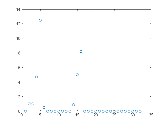
Tuning the regularization parameter usually improves the results. Suppose that, after tuning λ using cross-validation as in Tune Regularization Parameter in NCA for Regression, the best λ value found is 0.0035. Refit the nca model using this λ value and stochastic gradient descent as the solver. Compute the prediction loss.

nca3 = refit(nca2,FitMethod="exact",Lambda=0.0035, ...
    Solver="sgd");
L3 = loss(nca3,Xtest,ytest)
L3 = 0.0573

Plot the feature weights.

plot(nca3.FeatureWeights,"o")

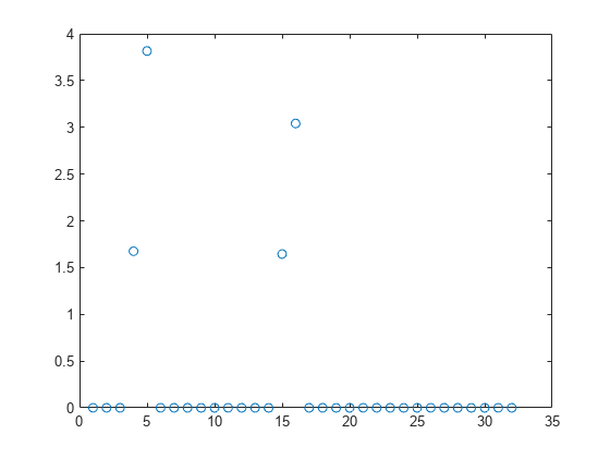
After tuning the regularization parameter, the loss decreased even more and the software identified four of the features as relevant.

References

[1] Rasmussen, C. E., R. M. Neal, G. E. Hinton, D. van Camp, M. Revow, Z. Ghahramani, R. Kustra, and R. Tibshirani. The DELVE Manual, 1996, https://mlg.eng.cam.ac.uk/pub/pdf/RasNeaHinetal96.pdf

[2] https://www.cs.toronto.edu/~delve/data/datasets.html

Input Arguments

collapse all

Neighborhood component analysis model or classification, specified as a FeatureSelectionNCARegression object.

Name-Value Arguments

Specify optional pairs of arguments as Name1=Value1,...,NameN=ValueN, where Name is the argument name and Value is the corresponding value. Name-value arguments must appear after other arguments, but the order of the pairs does not matter.

Example: refit(mdl,Lambda=0.01) refits the model mdl with a lambda value of 0.01.

Fitting Options

collapse all

Method for fitting the model, specified as one of the following.

  • "exact" — Performs fitting using all of the data.

  • "none" — No fitting. Use this option to evaluate the generalization error of the NCA model using the initial feature weights supplied in the call to fsrnca.

  • "average" — The function divides the data into partitions (subsets), fits each partition using the exact method, and returns the average of the feature weights. You can specify the number of partitions using the NumPartitions name-value argument.

Example: FitMethod="none"

Regularization parameter, specified as a nonnegative scalar value.

For n observations, the best Lambda value that minimizes the generalization error of the NCA model is expected to be a multiple of 1/n

Example: Lambda=0.01

Data Types: double | single

Solver type for estimating feature weights, specified as one of the following.

  • "lbfgs" — Limited memory BFGS (Broyden-Fletcher-Goldfarb-Shanno) algorithm (LBFGS algorithm)

  • "sgd" — Stochastic gradient descent

  • "minibatch-lbfgs" — Stochastic gradient descent with LBFGS algorithm applied to mini-batches

Example: Solver="minibatch-lbfgs"

Initial feature weights, specified as a p-by-1 vector of real positive scalar values.

Data Types: double | single

Indicator for verbosity level for the convergence summary display, specified as one of the following.

  • 0 — No convergence summary

  • 1 — Convergence summary including iteration number, norm of the gradient, and objective function value.

  • >1 — More convergence information depending on the fitting algorithm

    When using solver "minibatch-lbfgs" and verbosity level >1, the convergence information includes iteration log from intermediate mini-batch LBFGS fits.

Example: Verbose=2

Data Types: double | single

LBFGS or Mini-Batch LBFGS Options

collapse all

Relative convergence tolerance on the gradient norm for solver lbfgs, specified as a positive real scalar value.

Example: GradientTolerance=0.00001

Data Types: double | single

SGD or Mini-Batch LBFGS Options

collapse all

Initial learning rate for solver sgd, specified as a positive scalar value.

When using solver type "sgd", the learning rate decays over iterations starting with the value specified for InitialLearningRate.

Example: InitialLearningRate=0.8

Data Types: double | single

Maximum number of passes for solver "sgd" (stochastic gradient descent), specified as a positive integer value. Every pass processes size(mdl.X,1) observations.

Example: PassLimit=10

Data Types: double | single

SGD or LBFGS or Mini-Batch LBFGS Options

collapse all

Maximum number of iterations, specified as a positive integer.

Example: IterationLimit=250

Data Types: double | single

Output Arguments

collapse all

Neighborhood component analysis model or classification, returned as a FeatureSelectionNCARegression object. You can either save the results as a new model or update the existing model as mdl = refit(mdl,Name=Value).

Version History

Introduced in R2016b