ee_getPowerLossTimeSeries
Calculate dissipated power losses and switching losses, and return time series data
Syntax
Description
lossesCell = ee_getPowerLossTimeSeries(node)
Before you call this function, you must have the simulation log variable in your current workspace. Create the simulation log variable by simulating the model with data logging turned on, or load a previously saved variable from a file.
The ee_getPowerLossTimeSeries function calculates dissipated power
losses for each block that has a power_dissipated variable. All blocks in
the Semiconductor Devices library, as well as some other blocks, have an internal variable
called power_dissipated, which represents the instantaneous power
dissipated by the block. Some blocks have more than one power_dissipated
variable, depending on their configuration. For example, the N-Channel MOSFET
block has separate power_dissipated logging nodes for the MOSFET, the
gate resistor, and for the source and drain resistors if they have nonzero resistance
values. The function sums all these losses and provides the power loss value for all of the
blocks as functions of time.
Note
The power_dissipated internal variable does not report dynamic
losses incurred from semiconductor switching or magnetic hysteresis.
Three different variables, lastTurnOnLoss,
lastTurnOffLoss, and lastReverseRecoveryLoss
report the switching losses.
Switching losses are losses associated with the transition of the semiconductor switch
from its on-state to its off-state and vice versa, and also with the energy dissipated during
a reverse recovery event. They are frequency dependent. The
ee_getPowerLossTimeSeries function returns the switching losses at
each switching event and expresses them in joules.
These blocks in the Semiconductors & Converters library support the calculation of switching losses and reverse recovery losses, when applicable:
If node is the name of the simulation log variable, then the table
contains the data for all the blocks in the model that dissipate power (that is, contain at
least one power_dissipated variable). If node is the
name of a node in the simulation data tree, then the table contains the data only for the
blocks within that node.
lossesCell = ee_getPowerLossTimeSeries(node,startTime,endTime)startTime to endTime. If
startTime is equal to endTime, the interval is
effectively zero and the function returns the instantaneous power for the time step that
occurs at that moment. If you omit these two input arguments, the function returns data over
the whole simulation time.
lossesCell = ee_getPowerLossTimeSeries(node,startTime,...

endTime,intervalWidth)startTime to endTime, averaged over the time
intervalWidth. If you omit the intervalWidth, or
set it to 0, the function returns the instantaneous data, without averaging. If you omit all
three optional arguments, the function returns the instantaneous data over the whole
simulation time.
[
calculates dissipated power losses for blocks in a model, based on logged simulation data,
and returns the time series data, lossesCell, switchingLosses] = ee_getPowerLossTimeSeries(node)lossesCell, for each block and
a cell array, switchingLosses, with the switching losses of each
device.
If there are no switching losses appear, the switchingLosses
output is an empty cell array.
Examples
This example shows how to calculate instantaneous losses based on the power dissipated and return the time series data for all time steps in the entire simulation time using the ee_getPowerLossTimeSeries function.
Open the model. At the MATLAB® command prompt, enter:
model = 'ClassEDCDCConverter';
open_system(model)
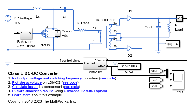
This example model has data logging enabled. Run the simulation and create the simulation log variable.
sim(model)
The simulation log variable simlog_ClassEDCDCConverter is saved in your current workspace.
Calculate dissipated power losses and return the time series data in cell array.
lossesCell = ee_getPowerLossTimeSeries(simlog_ClassEDCDCConverter)
lossesCell =

  9×2 cell array

    {'ClassEDCDCConverter.D1'         }    {100264×3 double}
    {'ClassEDCDCConverter.Cout'       }    {100264×3 double}
    {'ClassEDCDCConverter.R_Load.Res…'}    {100264×3 double}
    {'ClassEDCDCConverter.Ls'         }    {100264×3 double}
    {'ClassEDCDCConverter.LDMOS'      }    {100264×3 double}
    {'ClassEDCDCConverter.R_Trans.Re…'}    {100264×3 double}
    {'ClassEDCDCConverter.D2'         }    {100264×3 double}
    {'ClassEDCDCConverter.Behavioral…'}    {100264×3 double}
    {'ClassEDCDCConverter.Cs'         }    {100264×3 double}
View the time series data. From the workspace, open the lossesCell cell array, then open the numeric array for the diode block, ClassEDCDCConverter.D1.
The first two columns contain the interval start and end time. The third column contains the power loss data.
Plot the data.
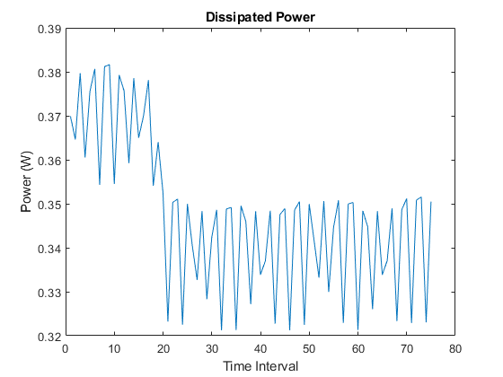
plot(lossesCell{1, 2}(:,end))
title('Dissipated Power')
xlabel('Time Interval')
ylabel('Power (W)')
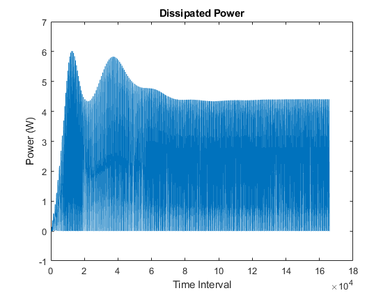
This example shows how to calculate instantaneous losses based on the power dissipated and return the time series data for all time steps in a specific time period using the ee_getPowerLossTimeSeries function.
Open the model. At the MATLAB® command prompt, enter:
model = 'ClassEDCDCConverter';
open_system(model)

This example model has data logging enabled. Run the simulation and create the simulation log variable.
sim(model)
The simulation log variable simlog_ClassEDCDCConverter is saved in your current workspace.
The model simulation time (t) is 1/8000 seconds. Calculate dissipated power losses and return the time series data in cell array for the second half of the simulation cycle, when t is between 1/16000 and 1/8000 seconds.
lossesCell = ee_getPowerLossTimeSeries(simlog_ClassEDCDCConverter,1/16000,1/8000)
lossesCell =

  9×2 cell array

    {'ClassEDCDCConverter.D1'         }    {49382×3 double}
    {'ClassEDCDCConverter.Cout'       }    {49382×3 double}
    {'ClassEDCDCConverter.R_Load.Res…'}    {49382×3 double}
    {'ClassEDCDCConverter.Ls'         }    {49382×3 double}
    {'ClassEDCDCConverter.LDMOS'      }    {49382×3 double}
    {'ClassEDCDCConverter.R_Trans.Re…'}    {49382×3 double}
    {'ClassEDCDCConverter.D2'         }    {49382×3 double}
    {'ClassEDCDCConverter.Behavioral…'}    {49382×3 double}
    {'ClassEDCDCConverter.Cs'         }    {49382×3 double}
View the time series data. From the workspace, open the lossesCell cell array, then open the array for the diode1 block, ClassEDCDCConverter.D1.
The first two columns contain the interval start and end time. The third column contains the power loss data.
Plot the data.
plot(lossesCell{1, 2}(:,end))
title('Dissipated Power')
xlabel('Time Interval')
ylabel('Power (W)')
This example shows how to calculate losses based on the power dissipated and return the time series data for a specific time period with averaging applied over intervals of a specified width.
Open the model. At the MATLAB® command prompt, enter:
model = 'PushPullBuckCCM';
open_system(model)
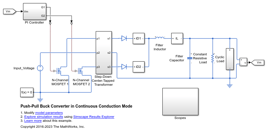
This example model has data logging enabled. Run the simulation and create the simulation log variable.
sim(model)
The simulation log variable simlog_PushPullBuckCCM is saved in your current workspace.
The model simulation time (t) is 0.04 seconds. Calculate the average dissipated power losses for 2.66e-4 s intervals and return the time series data in cell array for the period when simulation time, t, is 0.02-0.04 seconds.
lossesCell = ee_getPowerLossTimeSeries(simlog_PushPullBuckCCM,0.02,0.04,2.66e-4)
lossesCell =

  12×2 cell array

    {'PushPullBuckCCM.Filter_Capacit…'}    {75×3 double}
    {'PushPullBuckCCM.Filter_Inductor'}    {75×3 double}
    {'PushPullBuckCCM.Constant_Resis…'}    {75×3 double}
    {'PushPullBuckCCM.N_Channel_MOSF…'}    {75×3 double}
    {'PushPullBuckCCM.N_Channel_MOSF…'}    {75×3 double}
    {'PushPullBuckCCM.Diode.Diode'    }    {75×3 double}
    {'PushPullBuckCCM.Diode1.Diode'   }    {75×3 double}
    {'PushPullBuckCCM.Step_Down_Cent…'}    {75×3 double}
    {'PushPullBuckCCM.Step_Down_Cent…'}    {75×3 double}
    {'PushPullBuckCCM.Step_Down_Cent…'}    {75×3 double}
    {'PushPullBuckCCM.Step_Down_Cent…'}    {75×3 double}
    {'PushPullBuckCCM.Step_Down_Cent…'}    {75×3 double}
View the time series data. From the workspace, open the lossesCell cell array, then open the double numeric array for the PushPullBuckCCM.Diode
The first two columns contain the interval start and end time. The third column contains the power loss data. In this case, to use averaging intervals that are equal in width to 2.66e-4 seconds, the function adjusts the start time for the first interval from the specified value of 0.02 seconds to a value of 0.04 seconds. There are 75 intervals of 2.66e-4 seconds.
Plot the data.
plot(lossesCell{6, 2}(:,end))
title('Dissipated Power')
xlabel('Time Interval')
ylabel('Power (W)')
Input Arguments
Simulation log workspace variable, or a node within this variable,
that contains the logged model simulation data, specified as a Node object.
You specify the name of the simulation log variable by using the Workspace
variable name parameter on the Simscape pane
of the Configuration Parameters dialog box. To specify a node within
the simulation log variable, provide the complete path to that node
through the simulation data tree, starting with the top-level variable
name.
If node is the name of the simulation log
variable, then the table contains the data for all blocks in the model
that contain power_dissipated variables. If node is
the name of a node in the simulation data tree, then the table contains
the data only for:
Blocks or variables within that node
Blocks or variables within subnodes at all levels of the hierarchy beneath that node
Example: simlog.Cell1.MOS1
Start of the time interval for calculating the power loss time
series, specified as a real number, in seconds. startTime must
be greater than or equal to the simulation Start time and
less than endTime.
Data Types: double
End of the time interval for calculating the power loss time
series, specified as a real number, in seconds. endTime must
be greater than startTime and less than or equal
to the simulation Stop time.
Data Types: double
Size of the time interval for calculating the average power
dissipation, specified as a real number, in seconds. If specified,
the function returns data for time steps from startTime to endTime,
averaged over the intervalWidth. If you omit the intervalWidth argument,
or set it to 0, the function returns the instantaneous data, without
averaging. If all the optional arguments are omitted, the function
returns the instantaneous data over the whole simulation time.
If the time between the specified startTime and endTime is
not an integer multiple of intervalWidth, the
function adjusts the start time. The figure shows how the function
adjusts the start time to ensure that width of each time interval
that the dissipated power is averaged over is equal to the specified intervalWidth.
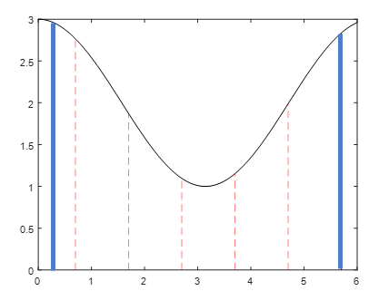
The black line is an example of the instantaneous power_dissipated variables
summed over all elements in an individual block. The simulation runs
for 6 seconds. The startTime and endTime are
indicated by the solid blue lines. The intervalWidth is
set to 1 second. There are five intervals as indicated by the red
dashed lines. The right-most edge of the last interval coincides with endTime.
The left-most edge of the first interval is always greater than or
equal to startTime. The edge is equal to startTime only
if (endTime -startTime)/intervalWidth is
an integer. The output in this case consists of five values for the
averaged power dissipation, one point for each time period. The function
outputs the actual start and stop times in the tabulated output data.
Example: 1.1e-3
Data Types: double
Output Arguments
Version History
Introduced in R2017a