Real-Time Signal Logging and Parameter Tuning

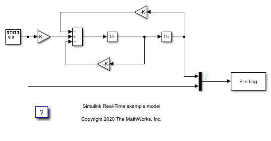
This example shows how to use real-time signal logging and parameter tuning with Simulink® Real-Time™. After the example builds the model and downloads the real-time application, slrt_ex_param_tuning, to the target computer, the example executes multiple runs and tunes the gain 'Gain1/Gain' parameter before each run. The gain sweeps from 0.1 to 0.7 in steps of 0.05.

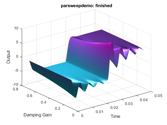
The example uses a Simulink Real-Time File Log block to capture signals of interest during each application run. The logged signals are uploaded to the development computer and plotted. A 3-D plot of the oscillator output versus time versus gain is displayed.

Create Target Object and Connect

Create a Target object for the default target computer and connect to the target computer. In the Command Window, type:

tg = slrealtime;
connect(tg);

Open, Build, and Download Model to the Target Computer

Open the model, slrt_ex_param_tuning. The model configuration parameters select the system target file (STF) that corresponds to the connected target computer, tg. Building the model creates a real-time application, slrt_ex_param_tuning.mldatx, that runs on the target computer.

model = 'slrt_ex_param_tuning';
open_system(model);
modelSTF = getSTFName(tg);
set_param(model,"SystemTargetFile",modelSTF);
set_param(model,'RTWVerbose','off');
set_param(model,'StopTime','0.2');

Build the model and download the real-time application, slrt_ex_param_tuning.mldatx, to the target computer.

• Configure for a non-Verbose build.

• Build and download application.

evalc('slbuild(model)');
load(tg,model);

Run Model, Sweep 'Gain' Parameter, Plot Logged Data

This code accomplishes several tasks.

Task 1: Create Target Object

Create the MATLAB® variable, tg, that contains the Simulink Real-Time target object. This object lets you communicate with and control the target computer.

• Create a Simulink Real-Time target object.

• Set stop time to 0.2s.

Task 2: Run the Model and Plot Results

Run the model, sweeping through and changing the gain (damping parameter) before each run. Plot the results for each run.

• If no plot figure exist, create the figure.

• If the plot figure exist, make it the current figure.

Task 3: Loop over damping factor z

• Set damping factor (Gain1/Gain).

• Start run of the real-time application.

• Store output data in outp, y, and t variables.

• Plot data for current run.

Task 4: Create 3-D Plot (Oscillator Output vs. Time vs. Gain)

• Loop over damping factor.

• Create a plot of oscillator output versus time versus gain.

• Create 3-D plot.

figh = findobj('Name', 'parsweepdemo');
if isempty(figh)
  figh = figure;
  set(figh, 'Name', 'parsweepdemo', 'NumberTitle', 'off');
else
  figure(figh);
end
y = []; flag = 0;
for z = 0.1 : 0.05 : 0.7
  if isempty(find(get(0, 'Children') == figh, 1))
      flag = 1;
      break;
  end
  load(tg,model);
  tg.setparam([model '/Gain1'],'Gain',2 * 1000 * z);
  tg.start('AutoImportFileLog',true, 'ExportToBaseWorkspace', true);
  pause(0.4);
  outp = logsOut{1}.Values;
  y    = [y,outp.Data(:,1)];
  t    = outp.Time;
  plot(t,y);
  set(gca, 'XLim', [t(1), t(end)], 'YLim', [-10, 10]);
  title(['parsweepdemo: Damping Gain = ', num2str(z)]);
  xlabel('Time'); ylabel('Output');
  drawnow;
end
if ~flag
  delete(gca);
  surf(t(1 : 200), 0.1 : 0.05 : 0.7, y(1 : 200, :)');
  colormap cool
  shading interp
  h = light;
  set(h, 'Position', [0.0125, 0.6, 10], 'Style', 'local');
  lighting gouraud
  title('parsweepdemo: finished');
  xlabel('Time'); ylabel('Damping Gain'); zlabel('Output');
end

  Importing Log file 1 of 1 ...
  Importing Log file 1 of 1 ...
  Importing Log file 1 of 1 ...
  Importing Log file 1 of 1 ...
  Importing Log file 1 of 1 ...
  Importing Log file 1 of 1 ...
  Importing Log file 1 of 1 ...
  Importing Log file 1 of 1 ...
  Importing Log file 1 of 1 ...
  Importing Log file 1 of 1 ...
  Importing Log file 1 of 1 ...
  Importing Log file 1 of 1 ...
  Importing Log file 1 of 1 ...

Close Model

When done, close the model.

bdclose(model);