Modeling Mechanical Position-Based Translational Systems
Intended Applications
The Translational library contains basic elements, such as mass, spring, damper, as well as sources and sensors. Use these blocks to model mechanical translational systems where it is important to know the component positions, for example, valve component assemblies.
The main benefits of the position-based domain are:
You can easily track positions and lengths of parts. This is especially useful for models with multiple blocks where behavior depends on position, such as spring and hard stop blocks. In the non-position-based mechanical translational domain, you must explicitly initialize the lengths, independently in each block, while the position-based domain synchronizes the positions automatically.
You can easily set up and intuitively interpret the directions of forces and velocities.
You can apply the effects of gravity to the entire network. The library contains the Mechanical Translational Properties (PB) block, which specifies the global parameters related to gravity for all the blocks in the attached circuit. This is especially useful when the model has many mass blocks with friction.
The library also contains the Interface (PB-Translational) block that allows connections between position-based and non-position-based mechanical translational ports. Use this block to connect the position-based Translational library blocks to blocks in other libraries, such as Mechanisms or Fluids.
Network Variables
The domain has two Across variables (position and velocity) and only one Through
variable (force). Therefore, the domain equations section contains one
equation that establishes the mathematical relationship between the position and velocity,
der(x) = v. For more information, see Domain Equations.
Position-Based Modeling Framework
In a position-based translational domain, blocks have a fixed orientation aligned with the global positive direction. Imagine all parts assembled on a rail.

Things to keep in mind:
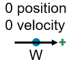
On the canvas, the Translational World (PB) block sets the absolute zero position and velocity in the model.
Model has a global positive direction.
All the blocks have a positive direction, which always aligns with the global positive direction. The global positive direction is determined when you place the first two-port block, External Force Source (PB) block, or External Translational Velocity Source (PB) block in the model. The External Force Source (PB) and External Translational Velocity Source (PB) blocks have one port. For these blocks, the positive direction is indicated by the arrow on the block icon.
For example, in the previous illustration, the global positive direction is from left to right. In your mental model, you can map the global positive direction of the model to represent left, right, up, or down.
Blocks can move only in the positive or negative direction. If you rotate a block on the canvas, it affects only the schematic view. For more information, see Difference Between Schematic View and Physical View.
Some blocks have length, specified as a block parameter or high-priority variable target. Other blocks are assumed to have zero length. When you place the blocks in the model and connect them, the software uses the block lengths to calculate the positions of all the block ports with respect to the absolute zero (the Translational World (PB) block), as shown in the illustration.
For example, in the previous illustration, you connect the blocks and specify the lengths, l1, l2, and l4. The software computes the values of the global positions, p0, p1, p2, and p4, and sets the variable target l3 = l2.
Types of Blocks
The blocks in a position-based translational domain conceptually belong to several distinct types.
| Block Type | Conventions | Schematic Representation |
|---|---|---|
| World |
|
|
| Two-port blocks |
|
|
| One-port blocks |
|
|

Difference Between Schematic View and Physical View
In a position-based translational domain, it is important to differentiate the schematic view from the physical view. For example, these two models are identical.
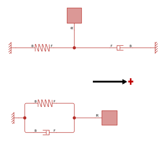
The top model shows a purely schematic view. The bottom model better represents the physical view, that is, the way the model actually looks in the physical world: with the spring and the damper located between the mass and the frame and acting in parallel. In this model, the global positive direction is easy to visualize.
The best practice is to draw model schematic on canvas in a way that is consistent with the physical view. Things to keep in mind:
Model canvas represents the schematic view. It shows block connectivity, not the part orientation.
When you rotate parts in the schematic view, the parts are not rotating in the physical world. For better intuitive understanding of the model, do not rotate parts relative to the global positive direction.
The Translational World (PB) block represents a single point in space. Therefore, in most situations it is consistent with the physical view to have only one Translational World (PB) block in a connected circuit.
Two-Port Block Orientation and Force Flow Conventions
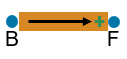
Two-port blocks in a position-based translational domain have length and a positive direction.
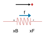
Typically, port F has a more positive position than port B and the length is positive. However, to support mechanisms that can invert and for simulation robustness, it is possible for two-port blocks to invert, in which case length becomes negative. Logged force f is always the force of port B acting on port F. The table summarizes the force flow conventions depending on the block orientation.
| Logged force, f, is positive | Logged force, f, is negative | |
|---|---|---|
| Length is positive (xF > xB) |
|
|
| Length is negative (xF < xB) |
|
|
Interpreting Logged Forces in Mass Blocks
In a position-based translational domain, there are several types of mass blocks. Point mass blocks have one port, R. Mass blocks with length have two ports, B and F. Both of these types have variants that let you model frictional effects.
| Point Mass | Mass with Length | |
|---|---|---|
| No Friction | Mass (PB) | Mass with Length (PB) |
| Frictional Effects | Mass with Friction (PB) | Mass with Length and Friction (PB) |
For more information on simulation data logging, see Data Logging. All mass blocks log the variables f and fmass. Mass blocks with frictional effects also log the variable ffriction. The force balance on the mass is:
fmass is the force that causes acceleration, . Positive fmass corresponds to a mass accelerating in the positive direction.
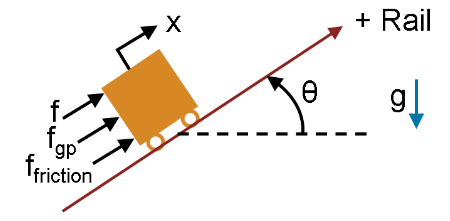
ffriction is the force of friction from the stationary rail acting on a mass. Negative ffriction acts in the negative direction and opposes a mass that moves in the positive direction. Positive ffriction acts in the positive direction and opposes a mass that moves in the negative direction.
fgp is the force proportional to the parallel component of gravitational acceleration, that is, to gravitational acceleration acting along the rail. For more information, see Mechanical Translational Properties (PB). Positive fgp corresponds to a negative incline angle and induces motion in the positive direction. Negative fgp corresponds to a positive incline angle and induces motion in the negative direction. Mass blocks do not log fgp because it is a constant value throughout the simulation.
f is force flow into the block, that is, net force of all the other mechanical components in the network acting on the mass. Positive f accelerates the mass in the positive direction, and negative f accelerates the mass in the negative direction.
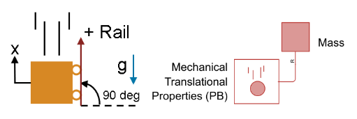
The Mechanical Translational Properties (PB) block specifies the gravitational acceleration and rail incline angle in the network. For example:
If the rail is vertical (β = 90 degrees) and the frictionless mass is motionless due to a support, then fmass = 0 and f = –fgp = m·g. f is the force of supports acting on the mass.
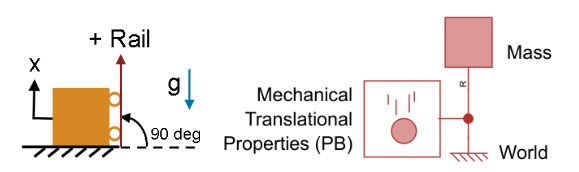
If the rail is vertical (β = 90 degrees) and the frictionless mass is accelerating in free fall, then fmass = fgp = –m·g and f = 0 N. That is, the other mechanical components in the network do not exert any force on the mass.