Measurement of Gain and Noise Figure Spectrum
This example shows how to use RF Blockset™ to measure the Gain and Noise Figure of an RF system over a given spectral range.
The example requires DSP System Toolbox™.
Introduction
In this example, a method for measuring the frequency-dependent gain and noise figure of an RF system is described. These spectral properties are measured for two RF systems; A single Low Noise Amplifier and the same amplifier when matched. The model used for the measurement is shown below:
model = 'GainNoiseMeasurementExample';
open_system(model);

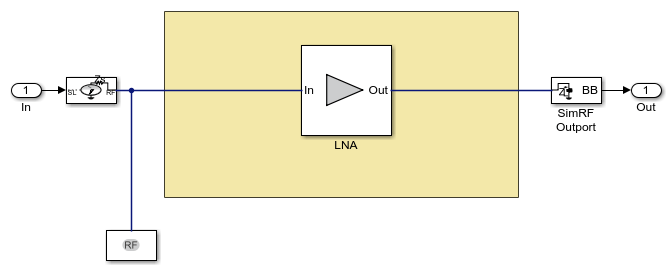
The model has two measurement units, each connected to a different subsystem containing the DUT. The upper measurement unit is connected to an unmatched LNA in the DUT subsystem with yellow background:
open_system([model '/DUT Unmatched']);
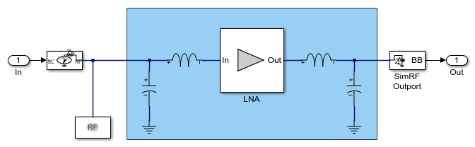
The lower measurement unit is connected to a matched LNA in the DUT subsystem with blue background:
open_system([model '/DUT Matched']);
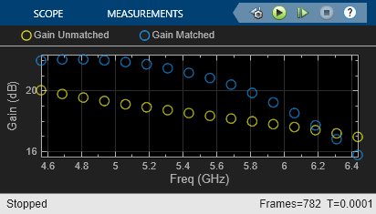
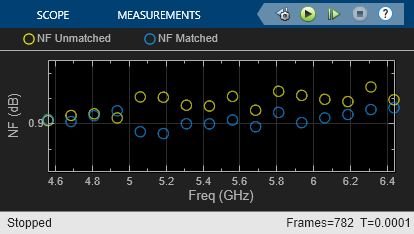
Each measurement unit outputs two vector signals representing the spectrums of the Gain and Noise Figure of the corresponding DUT and those are inputted into two Array Plot (DSP System Toolbox) blocks that plot the above properties versus frequency, comparing the unmatched and matched DUT systems. In the following sections, the matching network design process is described, the simulation results are given and compared with these expected from LNA and matching network properties. Finally, the procedure used within the measurement units to obtain the spectral Gain and Noise results is explained.
Design of the matching network
The matching network used in the matched DUT subsystem comprises a single stage L-C network that is designed following the same procedure as the one described in the RF Toolbox example Designing Matching Networks for Low Noise Amplifiers. Since the LNA used here is different, the design is described below
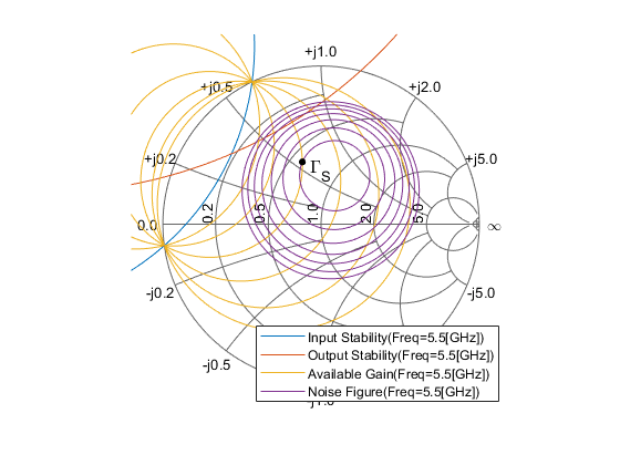
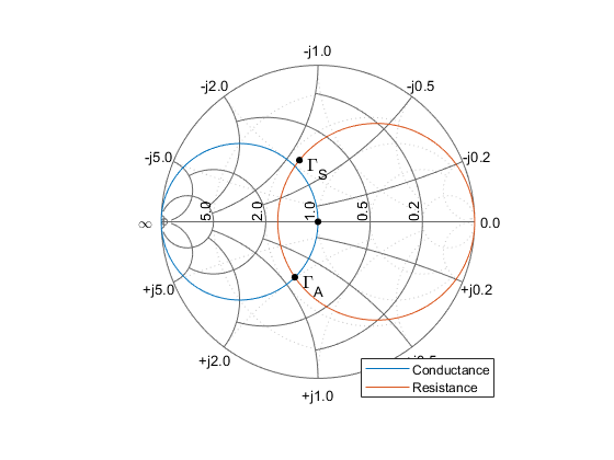
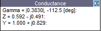
Initially, an rfckt.amplifier object is created to represent an Heterojunction Bipolar Transistor based low noise amplifier that is specified in the file, 'RF_HBT_LNA.S2P'. Then, the circle method of the rfckt.amplifier object is used to place the constant available gain and the constant noise figure circles on a Smith chart, and select an appropriate source reflection coefficient, GammaS, that provides a suitable compromise between gain and noise. The GammaS value chosen yields an available gain of Ga=21dB, and a noise figure of NF=0.9dB at the center frequency fc=5.5GHz:
unmatched_amp = read(rfckt.amplifier, 'RF_HBT_LNA.S2P');
fc = 5.5e9; % Center frequency (Hz)
circle(unmatched_amp,fc,'Stab','In','Stab','Out','Ga',15:2:25, ...
    'NF',0.9:0.1:1.5);

% Choose GammaS and show it on smith chart:
hold on
GammaS = 0.411*exp(1j*106.7*pi/180);
plot(GammaS,'k.','MarkerSize',16)
text(real(GammaS)+0.05,imag(GammaS)-0.05,'\Gamma_{S}','FontSize', 12, ...
    'FontUnits','normalized')
hLegend = legend('Location','SouthEast');
hLegend.String = hLegend.String(1:end-1);
hold off
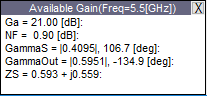
For the chosen GammaS, the following properties can be obtained:
% Normalized source impedance:
Zs = gamma2z(GammaS,1);

% Matching |GammaL| that is equal to the complex conjugate of
% |GammaOut| shown on the data tip:
GammaL = 0.595*exp(1j*135.0*pi/180);

% Normalized load impedance:
Zl = gamma2z(GammaL,1);
The input matching network consists of one shunt capacitor, Cin, and one series inductor, Lin. The Smith chart is used to find the component values. To do this, the constant conductance circle that crosses the center of the Smith chart and the constant resistance circle that crosses GammaS are plotted and the intersection points (Point  ) is found:
[~, hsm] = circle(unmatched_amp,fc,'G',1,'R',real(Zs));
hsm.Type = 'YZ';

% Choose GammaA and show points of interest on smith chart:
hold on
plot(GammaS,'k.','MarkerSize',16)
text(real(GammaS)+0.05,imag(GammaS)-0.05,'\Gamma_{S}','FontSize', 12, ...
    'FontUnits','normalized')
plot(0,0,'k.','MarkerSize',16)
GammaA = 0.384*exp(1j*(-112.6)*pi/180);
plot(GammaA,'k.','MarkerSize',16)
text(real(GammaA)+0.05,imag(GammaA)-0.05,'\Gamma_{A}','FontSize', 12, ...
    'FontUnits','normalized')
hLegend = legend('Location','SouthEast');
hLegend.String = hLegend.String(1:end-3);
hold off
Using the chosen GammaA, the input matching network components, Cin and Lin, are obtained:
% Obtain admittance Ya corresponding to GammaA:
Za = gamma2z(GammaA,1);
Ya = 1/Za;

% Using Ya, find Cin and Lin:
Cin = imag(Ya)/50/2/pi/fc
Lin = (imag(Zs) - imag(Za))*50/2/pi/fc
Cin =

   4.8145e-13


Lin =

   1.5218e-09
In a similar manner, the output matching network components are obtained using the intersection points (Point  ) between a constant conductance circle that crosses the center of the Smith chart and the constant resistance circle that crosses
 GammaL:
[hLine, hsm] = circle(unmatched_amp,fc,'G',1,'R',real(Zl));
hsm.Type = 'YZ';

% Choose GammaB and show points of interest on smith chart:
hold on
plot(GammaL,'k.','MarkerSize',16)
text(real(GammaL)+0.05,imag(GammaL)-0.05,'\Gamma_{L}','FontSize', 12, ...
    'FontUnits','normalized')
plot(0,0,'k.','MarkerSize',16)
GammaB = 0.612*exp(1j*(-127.8)*pi/180);
plot(GammaB,'k.','MarkerSize',16)
text(real(GammaB)+0.05,imag(GammaB)-0.05,'\Gamma_{B}','FontSize', 12, ...
    'FontUnits','normalized')
hLegend = legend('Location','SouthEast');
hLegend.String = hLegend.String(1:end-3);
hold off
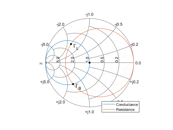
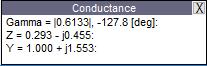
Using the chosen GammaB, the input matching network components, Cout and Lout, are obtained:
% Obtain admittance Yb corresponding to GammaB:
Zb = gamma2z(GammaB, 1);
Yb = 1/Zb;

% Using Yb, find Cout and Lout:
Cout = imag(Yb)/50/2/pi/fc
Cout =

   8.9651e-13
Lout = (imag(Zl) - imag(Zb))*50/2/pi/fc
Lout =

   1.2131e-09
Simulation results for gain and noise figure spectrum measurement model
The above input and output network component values are used in the simulation of the matched DUT in the gain and noise figure spectrum measurement model described earlier. The spectral results displayed in the Array Plot blocks are given below:
open_system([model '/Gain Spectrum']);
open_system([model '/Noise Figure Spectrum']);
sim(model, 1e-4);
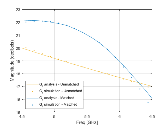
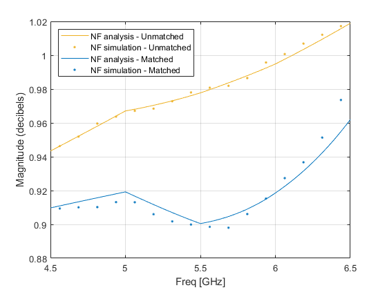
Next, the simulation results are compared with those expected analytically. To facilitate the comparison, the unmatched and matched amplifier networks are analyzed using RF Toolbox. In addition, as finer details are required, the simulation is run for a longer time. The results of the longer simulation are given in the file 'GainNoiseResults.mat'.
% Analyze unmatched amplifier
BW_analysis = 2e9; % Bandwidth of the analysis (Hz)
f_analysis = (-BW_analysis/2:1e6:BW_analysis/2)+fc;
analyze(unmatched_amp, f_analysis);

% Create and analyze an RF network for the matched amplifier
input_match = rfckt.cascade('Ckts', ...
    {rfckt.shuntrlc('C',Cin),rfckt.seriesrlc('L',Lin)});
output_match = rfckt.cascade('Ckts', ...
    {rfckt.seriesrlc('L',Lout),rfckt.shuntrlc('C',Cout)});
matched_amp = rfckt.cascade('ckts', ...
    {input_match,unmatched_amp,output_match});
analyze(matched_amp,f_analysis);

% Load results of a longer simulation
load 'GainNoiseResults.mat' f GainSpectrum NFSpectrum;

% Plot expected and simulated Transducer Gain
StdBlue = [0 0.45 0.74];
StdYellow = [0.93,0.69,0.13];
hLineUM = plot(unmatched_amp, 'Gt', 'dB');
hLineUM.Color = StdYellow;
hold on
plot(f, GainSpectrum(:,1), '.', 'Color', StdYellow);
hLineM = plot(matched_amp, 'Gt', 'dB');
hLineM.Color = StdBlue;
plot(f, GainSpectrum(:,2), '.', 'Color', StdBlue);
legend({'G_t analysis - Unmatched', ...
        'G_t simulation - Unmatched', ...
        'G_t analysis - Matched', ...
        'G_t simulation - Matched'}, 'Location','SouthWest');

% Plot expected and simulated Noise Figure
hFig = figure;
hLineUM = plot(unmatched_amp, 'NF', 'dB');
hLineUM.Color = StdYellow;
legend('Location','NorthWest')
hold on
plot(f, NFSpectrum(:,1), '.', 'Color', StdYellow);
hLineM = plot(matched_amp, 'NF', 'dB');
hLineM.Color = StdBlue;
plot(f, NFSpectrum(:,2), '.', 'Color', StdBlue);
legend({'NF analysis - Unmatched', ...
        'NF simulation - Unmatched', ...
        'NF analysis - Matched', ...
        'NF simulation - Matched'}, 'Location','NorthWest');
Operation of the measurement unit
The measurement unit produces an input signal, DUT_in, that is composed of zero-mean white noise and zero-variance impulse response signal. The latter is used to determine the frequency response of the DUT gain and together with the white noise determine the DUT noise figure. The measurement unit collects the DUT output signal, performs a windowed FFT on it and then facilitates statistical calculations to obtain the gain and the noise figure of the DUT.
open_system([model '/Noise and Gain Measurement'], 'force');
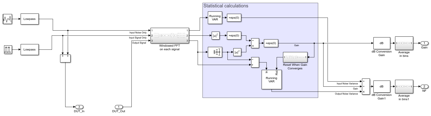
The statistical calculations are done in the area marked in blue. The calculations use three inputs in the frequency domain; Input Noise Only, Input Signal Only, and Output Signal. The Input Signal Only is compared with the mean of the Output Signal to determine the DUT's gain,  , at each frequency bin. The variance of the Output Signal, with mean signal removed, yields the output noise of the DUT system,
  , Together with the input noise fed to the DUT,
  , calculated by taking the variance of the Input Noise Only, the Noise Figure,
  , can be calculated using the following formula:
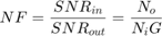
Where,  and
and  in the above equation are the Signal-to-Noise ratios at the input and output of the DUT. Finally, after conversion to decibels, the spectral results are divided into bins and averaged within them to facilitate faster convergence. Also, to improve the noise calculation convergence, the output noise variance is reset once the gain has reached convergence.
The properties affecting the operation of the measurement unit are specified in the block's mask parameter dialog box as shown below:
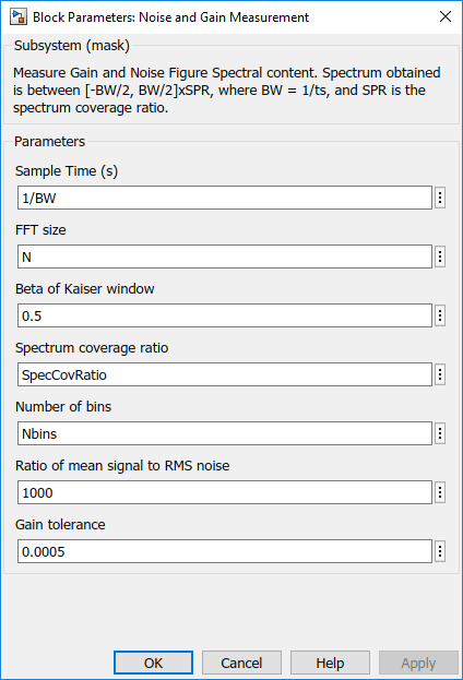
These parameters are described below:
Sample time - Sample time of the signal created by the measurement unit. The sample time also governs the total simulation bandwidth captured by the measurement unit.
FFT size - Number of FFT bins used to obtain the frequency domain representation of the signals within the measurement unit.
Beta of Kaiser window - The
 parameter of the Kaiser window used in all FFT calculations within the measurement unit. Increasing widens the mainlobe and decreases the amplitude of the sidelobes of the frequency response of the window.
Spectrum coverage ratio - Value between 0 and 1, representing the part of total simulation bandwidth processed by the measurement unit.
Number of bins - Number of output frequency bins in the Gain and NF signals created by the measurement unit. The FFT bins within the covered spectrum are re-distributed into those output bins. Multiple FFT bins falling into the same output bin are averaged.
Ratio of mean signal to RMS noise - The ratio of the mean signal amplitude to the RMS noise in the DUT_in signal created by the measurement unit. A large value improves the convergence of the DUT gain calculation, but reduces the accuracy of noise calculation due to numerical inaccuracies.
Gain tolerance - The threshold of gain variation relative to its average. When the threshold is hit, the gain is considered as converged, triggering a reset for the output noise calculation.
close(hFig);
bdclose(model);
clear model hLegend hsm hLine hLegend StdBlue StdYellow hLineUM hLineM hFig;
clear GammaS Zs GammaL Zl GammaA Za Ya GammaB Zb Yb;
clear unmatched_amp BW_analysis f_analysis input_match output_match matched_amp;
See Also
Amplifier | Configuration | Inport | Outport