SimBiology.gsa.ElementaryEffects
Object containing results from calculation of elementary effects for global sensitivity analysis (GSA)
Since R2021b
Description
The SimBiology.gsa.ElementaryEffects object contains GSA results
returned by sbioelementaryeffects. The object contains the computed elementary effects with
respect to parameter inputs.
Creation
Create a SimBiology.gsa.ElementaryEffects object using sbioelementaryeffects.
Properties
Flag to use the absolute values of elementary effects, specified as true or
false. By default, the function uses the absolute values of
elementary effects. Using nonabsolute values can average out when calculating the mean. For
details, see Elementary Effects for Global Sensitivity Analysis.
Data Types: logical
This property is read-only.
Time points at which elementary effects are computed, specified as a column numeric
vector. The property is [] if all observables are scalars.
Data Types: double
This property is read-only.
GSA results with elementary effects, specified as a structure array. The size of the array is params-by-observables, where params is the number of input parameters (sensitivity inputs) and observables is the number of observables (sensitivity outputs).
Each structure contains the following fields.
Parameter— Name of an input parameter, specified as a character vectorObservable— Name of an observable, specified as a character vectorMean— Mean of elementary effects, specified as a scalar or numeric vectorStandardDeviation— Standard deviation of elementary effects, specified as a scalar or numeric vector
If all observables are scalar, then the Mean and
StandardDeviation fields are specified as scalars. If any
observables are vectors, Mean and
StandardDeviation are numeric vectors of length
Time. If some observables are scalars and some are vectors,
scalar observables are scalar-expanded, where each time point has the same value.
Data Types: struct
This property is read-only.
Discretization level of the parameter domain, specified as a positive even integer. This
parameter defines a grid of equidistant points in the parameter domain, where each dimension
is discretized using Gridlevel+1
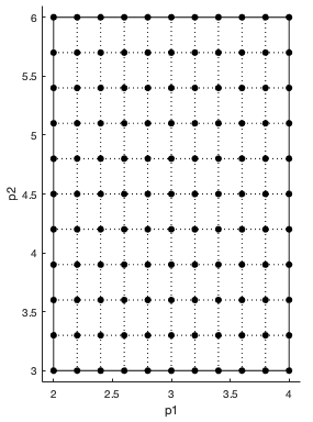
For details, see Elementary Effects for Global Sensitivity Analysis.
Data Types: double
This property is read-only.
Step size for computing elementary effects, specified as a positive integer between 1 and
GridLevel. The step size is measured in terms of grid points
between neighboring points. The following figure shows examples of different grid delta
values.
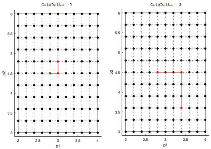
For details, see Elementary Effects for Global Sensitivity Analysis.
Data Types: double
This property is read-only.
Method to select sample points to compute elementary effects, specified as
"chain" or "radial". The
"chain" point selection uses the Morris method [1]. The
"radial" point selection uses the Sohier method [2]. For details, see
Elementary Effects for Global Sensitivity Analysis.
Data Types: double
This property is read-only.
Sampled parameter values, specified as a table. The table contains
(1+numel(params))*NumberSamples rows and
numel(params) columns.
sbioelementaryeffects uses blocks of
k+1 rows, where k is the
number of input params, to compute an elementary effect for each input parameter. The total number of these
blocks is equal to the total number of samples. You can get the block indices by running
kron((1:NumberSamples)',ones(numel(params)+1,1)). For details, see
Elementary Effects for Global Sensitivity Analysis.
Data Types: table
This property is read-only.
Names of model responses or observables, specified as a cell array of character vectors.
Data Types: char
This property is read-only.
Simulation information, such as simulation data and parameter samples, used for computing elementary effects, specified as a structure. The structure contains the following fields.
SimFunction—SimFunctionobject used for simulating model responses or observables.SimData—SimDataarray of size[NumberSamples,1], where NumberSamples is the number of samples. The array contains simulation results fromParameterSamples.OutputTimes— Numeric column vector containing the common time vector of allSimDataobjects.Bounds— Numeric matrix of size[params,2]. params is the number of input parameters. The first column contains the lower bounds and the second column contains the upper bounds for sensitivity inputs.DoseTables— Cell array of dose tables used for theSimFunctionevaluation.DoseTablesis the output ofgetTable(doseInput), where doseInput is the value specified for the'Doses'name-value pair argument in the call tosbiosobol,sbiompgsa, orsbioelementaryeffects. If no doses are applied, this field is set to[].ValidSample— Logical vector of size[NumberSamples,1]indicating whether a simulation for a particular sample failed. Resampling of the simulation data (SimData) can result inNaNvalues if the data is extrapolated. SuchSimDataare indicated as invalid.InterpolationMethod— Name of the interpolation method forSimData.SamplingMethod— Name of the sampling method used to drawParameterSamples.RandomState— Structure containing the state ofrngbefore drawingParameterSamples.
Data Types: struct
Object Functions
resample | Resample Sobol indices or elementary effects to new time vector |
addobservable | Compute Sobol indices or elementary effects for new observable expression |
removeobservable | Remove Sobol indices or elementary effects of observables |
addsamples | Add additional samples to increase accuracy of Sobol indices or elementary effects analysis |
plotData | Plot quantile summary of model simulations from global sensitivity analysis |
plot | Plot means and standard deviations of elementary effects |
bar | Plot magnitudes of means and standard deviations of elementary effects |
plotGrid | Plot parameter grid and points used to compute elementary effects |
Examples
Load the tumor growth model.
sbioloadproject tumor_growth_vpop_sa.sbprojGet a variant with estimated parameters and the dose to apply to the model.
v = getvariant(m1);
d = getdose(m1,'interval_dose');
Get the active configset and set the tumor weight as the response.
cs = getconfigset(m1);
cs.RuntimeOptions.StatesToLog = 'tumor_weight';
Simulate the model and plot the tumor growth profile.
sbioplot(sbiosimulate(m1,cs,v,d));
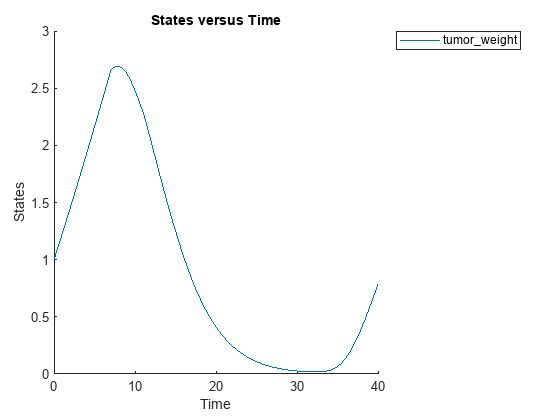
Perform global sensitivity analysis (GSA) on the model to find the model parameters that the tumor growth is sensitive to.
First, define model parameters of interest, which are involved in the pharmacodynamics of the tumor growth. Define the model response as the tumor weight.
modelParamNames = {'L0','L1','w0','k1'};
outputName = 'tumor_weight';
Then perform GSA by computing the elementary effects using sbioelementaryeffects. Use 100 as the number of samples and set ShowWaitBar to true to show the simulation progress.
rng('default');
eeResults = sbioelementaryeffects(m1,modelParamNames,outputName,Variants=v,Doses=d,NumberSamples=100,ShowWaitbar=true);
Show the median model response, the simulation results, and a shaded region covering 90% of the simulation results.
plotData(eeResults,ShowMedian=true,ShowMean=false);
![Figure contains an axes object. The axes object with xlabel time, ylabel [Tumor Growth].tumor indexOf w baseline eight contains 12 objects of type line, patch. These objects represent model simulation, 90.0% region, median value.](../../examples/simbio/win64/PerformGSAByComputingElementaryEffectsExample_02.png)
You can adjust the quantile region to a different percentage by specifying Alphas for the lower and upper quantiles of all model responses. For instance, an alpha value of 0.1 plots a shaded region between the 100*alpha and 100*(1-alpha) quantiles of all simulated model responses.
plotData(eeResults,Alphas=0.1,ShowMedian=true,ShowMean=false);
![Figure contains an axes object. The axes object with xlabel time, ylabel [Tumor Growth].tumor indexOf w baseline eight contains 12 objects of type line, patch. These objects represent model simulation, 80.0% region, median value.](../../examples/simbio/win64/PerformGSAByComputingElementaryEffectsExample_03.png)
Plot the time course of the means and standard deviations of the elementary effects.
h = plot(eeResults);
% Resize the figure.
h.Position(:) = [100 100 1280 800];![Figure contains 8 axes objects. Axes object 1 with xlabel time, ylabel std. of effects k1 contains an object of type line. Axes object 2 with xlabel time, ylabel mean of effects k1 contains an object of type line. Axes object 3 with ylabel std. of effects w0 contains an object of type line. Axes object 4 with ylabel mean of effects w0 contains an object of type line. Axes object 5 with ylabel std. of effects L1 contains an object of type line. Axes object 6 with ylabel mean of effects L1 contains an object of type line. Axes object 7 with title sensitivity output [Tumor Growth].tumor_weight, ylabel std. of effects L0 contains an object of type line. Axes object 8 with title sensitivity output [Tumor Growth].tumor_weight, ylabel mean of effects L0 contains an object of type line.](../../examples/simbio/win64/PerformGSAByComputingElementaryEffectsExample_04.png)
The mean of effects explains whether variations in input parameter values have any effect on the tumor weight response. The standard deviation of effects explains whether the sensitivity change is dependent on the location in the parameter domain.
From the mean of effects plots, parameters L1 and w0 seem to be the most sensitive parameters to the tumor weight before the dose is applied at t = 7. But, after the dose is applied, k1 and L0 become more sensitive parameters and contribute most to the after-dosing stage of the tumor weight. The plots of standard deviation of effects show more deviations for the larger parameter values in the later stage (t > 35) than for the before-dose stage of the tumor growth.
You can also display the magnitudes of the sensitivities in a bar plot. Each color shading represents a histogram representing values at different times. Darker colors mean that those values occur more often over the whole time course.
bar(eeResults);
![Figure contains an axes object. The axes object with title sensitivity output [Tumor Growth].tumor_weight, xlabel elementary effects, ylabel sensitivity input contains 18 objects of type patch, line. These objects represent mean, standard deviation.](../../examples/simbio/win64/PerformGSAByComputingElementaryEffectsExample_05.png)
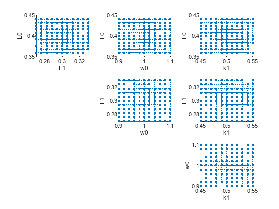
You can also plot the parameter grids and samples used to compute the elementary effects.
plotGrid(eeResults)
You can specify more samples to increase the accuracy of the elementary effects, but the simulation can take longer to finish. Use addsamples to add more samples.
eeResults2 = addsamples(eeResults,200);
The SimulationInfo property of the result object contains various information for computing the elementary effects. For instance, the model simulation data (SimData) for each simulation using a set of parameter samples is stored in the SimData field of the property. This field is an array of SimData objects.
eeResults2.SimulationInfo.SimData
   SimBiology SimData Array : 1500-by-1

   Index:    Name:         ModelName:         DataCount:
   1           -           Tumor Growth Model 1
   2           -           Tumor Growth Model 1
   3           -           Tumor Growth Model 1
   ...
   1500        -           Tumor Growth Model 1
You can find out if any model simulation failed during the computation by checking the ValidSample field of SimulationInfo. In this example, the field shows no failed simulation runs.
all(eeResults2.SimulationInfo.ValidSample)
ans = logical
   1
You can add custom expressions as observables and compute the elementary effects of the added observables. For example, you can compute the effects for the maximum tumor weight by defining a custom expression as follows.
% Suppress an information warning that is issued.
warnSettings = warning('off', 'SimBiology:sbservices:SB_DIMANALYSISNOTDONE_MATLABFCN_UCON');
% Add the observable expression.
eeObs = addobservable(eeResults2,'Maximum tumor_weight','max(tumor_weight)','Units','gram');
Plot the computed simulation results showing the 90% quantile region.
h2 = plotData(eeObs,ShowMedian=true,ShowMean=false);
h2.Position(:) = [100 100 1500 800];
![Figure contains 2 axes objects. Axes object 1 with ylabel Maximum tumor_weight contains 12 objects of type line, patch. One or more of the lines displays its values using only markers These objects represent model simulation, 90.0% region, median value. Axes object 2 with xlabel time, ylabel [Tumor Growth].tumor_weight contains 12 objects of type line, patch. These objects represent model simulation, 90.0% region, median value.](../../examples/simbio/win64/PerformGSAByComputingElementaryEffectsExample_07.png)
You can also remove the observable by specifying its name.
eeNoObs = removeobservable(eeObs,'Maximum tumor_weight');Restore the warning settings.
warning(warnSettings);
References
[1] Morris, Max D. “Factorial Sampling Plans for Preliminary Computational Experiments.” Technometrics 33, no. 2 (May 1991): 161–74.
[2] Sohier, Henri, Jean-Loup Farges, and Helene Piet-Lahanier. “Improvement of the Representativity of the Morris Method for Air-Launch-to-Orbit Separation.” IFAC Proceedings Volumes 47, no. 3 (2014): 7954–59.
Version History
Introduced in R2021b