predict
Simulate and evaluate fitted SimBiology model
Syntax
Description
[ returns simulation results
ynew,parameterEstimates]=
predict(resultsObj)ynew and parameter estimates
parameterEstimates of a fitted SimBiology® model.
[
returns simulation results ynew,parameterEstimates]=
predict(resultsObj,data,dosing)ynew and estimated parameter values
parameterEstimates from evaluating the fitted SimBiology
model using the specified data and dosing
information.
During simulations, predict uses the parameter values in the
resultsObj.ParameterEstimates property. Use this method when
you want to evaluate the fitted model and predict responses using new data and/or
dosing information.
[
simulates the fitted model and applies the specified variants to each
simulation.ynew,parameterEstimates]=
predict(resultsObj,data,dosing,'Variants',v)
Examples
This example uses the yeast heterotrimeric G protein model and experimental data reported by [1]. For details about the model, see the Background section in Parameter Scanning, Parameter Estimation, and Sensitivity Analysis in the Yeast Heterotrimeric G Protein Cycle.
Load the G protein model.
sbioloadproject gproteinStore the experimental data containing the time course for the fraction of active G protein.
time = [0 10 30 60 110 210 300 450 600]';
GaFracExpt = [0 0.35 0.4 0.36 0.39 0.33 0.24 0.17 0.2]';
Map the appropriate model component to the experimental data. In other words, indicate which species in the model corresponds to which response variable in the data. In this example, map the model parameter GaFrac to the experimental data variable GaFracExpt from grpData.
responseMap = 'GaFrac = GaFracExpt';Create a groupedData object based on the experimental data.
tbl = table(time,GaFracExpt);
grpData = groupedData(tbl);
Use an estimatedInfo object to define the model parameter kGd as a parameter to be estimated.
estimatedParam = estimatedInfo('kGd');Perform the parameter estimation.
fitResult = sbiofit(m1,grpData,responseMap,estimatedParam);
View the estimated parameter value of kGd.
fitResult.ParameterEstimates
ans=1×3 table
     Name      Estimate    StandardError
    _______    ________    _____________

    {'kGd'}    0.11307      3.4439e-05
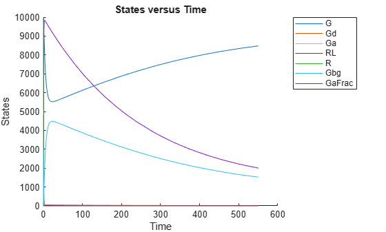
Suppose you want to simulate the fitted model using different output times than those in the training data. You can use the predict method to do so.
Create a new variable T with different output times.
T = [0;10;50;80;100;150;300;350;400;450;500;550];
Use the predict method to simulate the fitted model on the new time points. No dosing was specified when you first ran sbiofit. Hence, you cannot use any dosing information with the predict method, and an empty array must be specified as the third input argument.
ynew = predict(fitResult,T,[]);
Plot the simulated data with the new output times.
sbioplot(ynew);
This example shows how to estimate category-specific (such as young versus old, male versus female) PK parameters using the profile data from multiple individuals using a two-compartment model. The parameters to estimate are the volumes of central and peripheral compartment, the clearance, and intercompartmental clearance.
The synthetic data used in this example contains the time course of plasma concentrations of multiple individuals after a bolus dose (100 mg) measured at different times for both central and peripheral compartments. It also contains categorical variables, namely Sex and Age.
clear
load('sd5_302RAgeSex.mat');
Convert the data set to a groupedData object, which is the required data format for the fitting function sbiofit. A groupedData object allows you to set independent variable and group variable names (if they exist). Set the units of the ID, Time, CentralConc, PeripheralConc, Age, and Sex variables. The units are optional and only required for the UnitConversion feature, which automatically converts matching physical quantities to one consistent unit system.
gData = groupedData(data);
gData.Properties.VariableUnits = {'','hour','milligram/liter','milligram/liter','',''};
The IndependentVariableName and GroupVariableName properties have been automatically set to the Time and ID variables of the data.
gData.Properties
ans = struct with fields:
                Description: ''
                   UserData: []
             DimensionNames: {'Row'  'Variables'}
              VariableNames: {'ID'  'Time'  'CentralConc'  'PeripheralConc'  'Sex'  'Age'}
              VariableTypes: ["double"    "double"    "double"    "double"    "categorical"    "categorical"]
       VariableDescriptions: {}
              VariableUnits: {''  'hour'  'milligram/liter'  'milligram/liter'  ''  ''}
         VariableContinuity: []
                   RowNames: {}
           CustomProperties: [1×1 matlab.tabular.CustomProperties]
          GroupVariableName: 'ID'
    IndependentVariableName: 'Time'
For illustration purposes, use the first five individual data for training and the 6th individual data for testing.
trainData = gData([gData.ID < 6],:);
testData  = gData([gData.ID == 6],:);
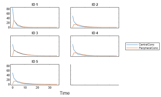
Display the response data for each individual in the training set.
sbiotrellis(trainData,'ID','Time',{'CentralConc','PeripheralConc'});
Use the built-in PK library to construct a two-compartment model with infusion dosing and first-order elimination where the elimination rate depends on the clearance and volume of the central compartment. Use the configset object to turn on unit conversion.
pkmd                                    = PKModelDesign;
pkc1                                    = addCompartment(pkmd,'Central');
pkc1.DosingType                         = 'Bolus';
pkc1.EliminationType                    = 'linear-clearance';
pkc1.HasResponseVariable                = true;
pkc2                                    = addCompartment(pkmd,'Peripheral');
model                                   = construct(pkmd);
configset                               = getconfigset(model);
configset.CompileOptions.UnitConversion = true;
Assume every individual receives a bolus dose of 100 mg at time = 0.
dose             = sbiodose('dose','TargetName','Drug_Central');
dose.StartTime   = 0;
dose.Amount      = 100;
dose.AmountUnits = 'milligram';
dose.TimeUnits   = 'hour';
The data contains measured plasma concentration in the central and peripheral compartments. Map these variables to the appropriate model components, which are Drug_Central and Drug_Peripheral.
responseMap = {'Drug_Central = CentralConc','Drug_Peripheral = PeripheralConc'};Specify the volumes of central and peripheral compartments Central and Peripheral, intercompartmental clearance Q12, and clearance Cl_Central as parameters to estimate. The estimatedInfo object lets you optionally specify parameter transforms, initial values, and parameter bounds. Since both Central and Peripheral are constrained to be positive, specify a log-transform for each parameter.
paramsToEstimate    = {'log(Central)', 'log(Peripheral)', 'Q12', 'Cl_Central'};
estimatedParam      = estimatedInfo(paramsToEstimate,'InitialValue',[1 1 1 1]);
Use the 'CategoryVariableName' property of the estimatedInfo object to specify which category to use during fitting. Use 'Sex' as the group to fit for the clearance Cl_Central and Q12 parameters. Use 'Age' as the group to fit for the Central and Peripheral parameters.
estimatedParam(1).CategoryVariableName = 'Age';
estimatedParam(2).CategoryVariableName = 'Age';
estimatedParam(3).CategoryVariableName = 'Sex';
estimatedParam(4).CategoryVariableName = 'Sex';
categoryFit = sbiofit(model,trainData,responseMap,estimatedParam,dose)
categoryFit =
  OptimResults with properties:

                   ExitFlag: 1
                     Output: [1×1 struct]
                  GroupName: []
                       Beta: [8×5 table]
         ParameterEstimates: [20×6 table]
                          J: [40×8×2 double]
                       COVB: [8×8 double]
           CovarianceMatrix: [8×8 double]
                          R: [40×2 double]
                        MSE: 0.1047
                        SSE: 7.5349
                    Weights: []
              LogLikelihood: -19.0159
                        AIC: 54.0318
                        BIC: 73.0881
                        DFE: 72
             DependentFiles: {1×3 cell}
                       Data: [40×6 groupedData]
    EstimatedParameterNames: {'Central'  'Peripheral'  'Q12'  'Cl_Central'}
             ErrorModelInfo: [1×3 table]
         EstimationFunction: 'lsqnonlin'
When fitting by category (or group), sbiofit always returns one results object, not one for each category level. This is because both male and female individuals are considered to be part of the same optimization using the same error model and error parameters, similarly for the young and old individuals.
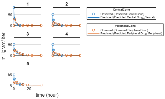
Plot the category-specific estimated results. For the Cl_Central and Q12 parameters, all males had the same estimates, and similarly for the females. For the Central and Peripheral parameters, all young individuals had the same estimates, and similarly for the old individuals.
plot(categoryFit);
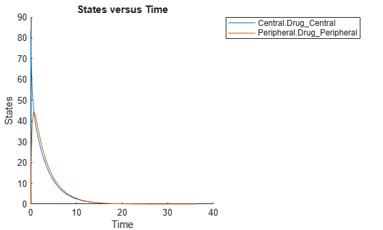
As for testing purposes, simulate the responses of the 6th individual who is an old male. Since you have estimated one set of parameters for the Age category (young versus old), and another set for Sex category (male versus female), you can simulate the responses of an old male even though there is no such individual in the training data.
Use the predict method to simulate the responses. ynew contains simulation data and paramestim contains parameter estimates used during simulation.
[ynew,paramestim] = predict(categoryFit,testData,dose);
Plot the simulated responses of the old male.
sbioplot(ynew);
The paramestim variable contains the estimated parameters used by the predict method. The parameter estimates for corresponding categories were obtained from the categoryFit.ParameterEstimates property. Specifically, Central and Peripheral parameter estimates are obtained from the Old group, and Q12 and Cl_Central parameter estimates are obtained from the Male group.
paramestim
paramestim=4×6 table
         Name         Estimate    StandardError    Group    CategoryVariableName    CategoryValue
    ______________    ________    _____________    _____    ____________________    _____________

    {'Central'   }     1.1993       0.0046483        6            {'Age'}               Old
    {'Peripheral'}    0.55195        0.015098        6            {'Age'}               Old
    {'Q12'       }     1.4969        0.074321        6            {'Sex'}               Male
    {'Cl_Central'}    0.56363       0.0072862        6            {'Sex'}               Male
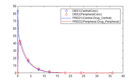
Overlay the experimental results on the simulated data.
figure;
plot(testData.Time,testData.CentralConc,'LineStyle','none','Marker','d','MarkerEdgeColor','b');
hold on
plot(testData.Time,testData.PeripheralConc,'LineStyle','none','Marker','d','MarkerEdgeColor','r');
plot(ynew.Time,ynew.Data(:,1),'b');
plot(ynew.Time,ynew.Data(:,2),'r');
hold off
legend({'OBS1(CentralConc)','OBS2(PeripheralConc)',...
        'PRED1(Central.Drug\_Central)','PRED2(Peripheral.Drug\_Peripheral)'});
Input Arguments
Output Arguments
References
[1] Yi, T-M., Kitano, H., and Simon, M. (2003). A quantitative characterization of the yeast heterotrimeric G protein cycle. PNAS. 100, 10764–10769.
Version History
Introduced in R2014a